E01 — 12-slot / 10-pole surface-PM synchronous machine

← Back to the examples

What you need to run it: the Python API and the Machines module. Opening the model and reading results that are already there never requires a licence.

At a glance

Quantity	Value	Unit
Speed	2000	rpm
Electrical frequency	166.7	Hz
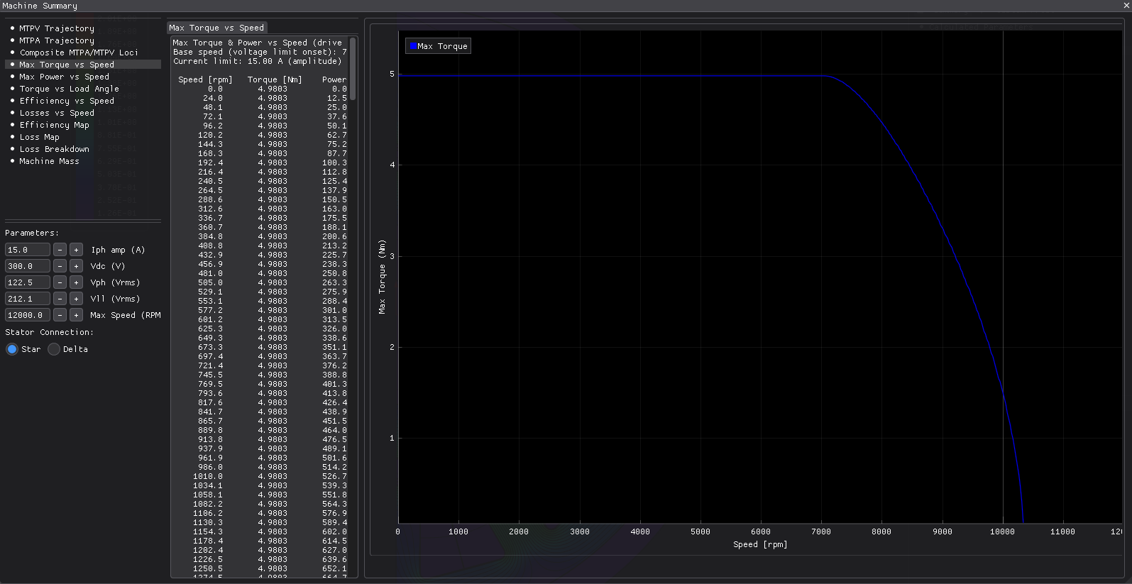
Average torque	4.956	N·m
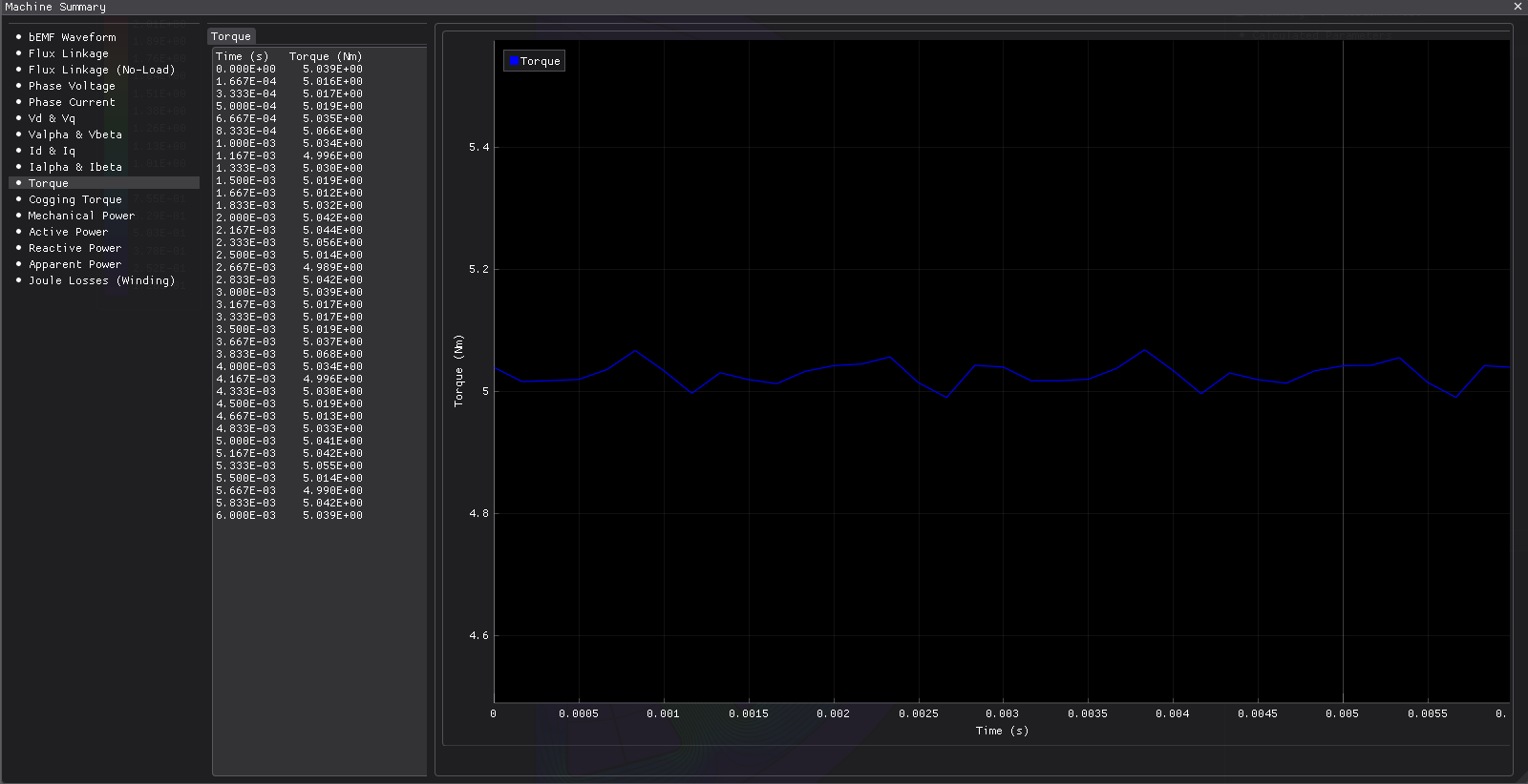
Torque ripple	3.7	%
Cogging torque, peak-peak	0.176	N·m
Back-EMF, RMS	34.5	V
Mechanical power	1.038	kW
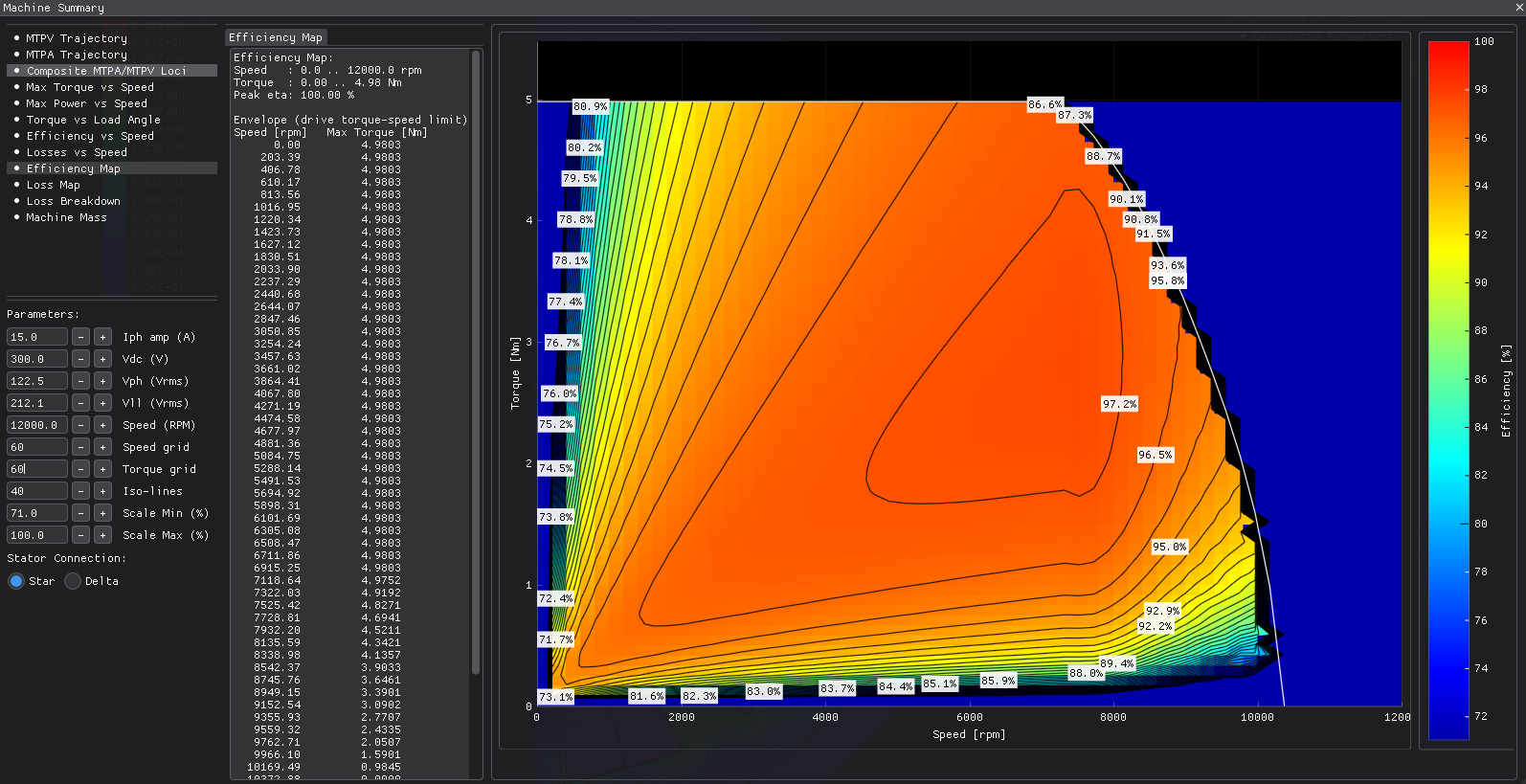
Efficiency	91.65	%
Power factor	0.966	—
Total losses	94.5	W
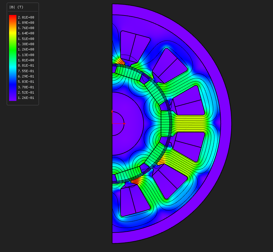
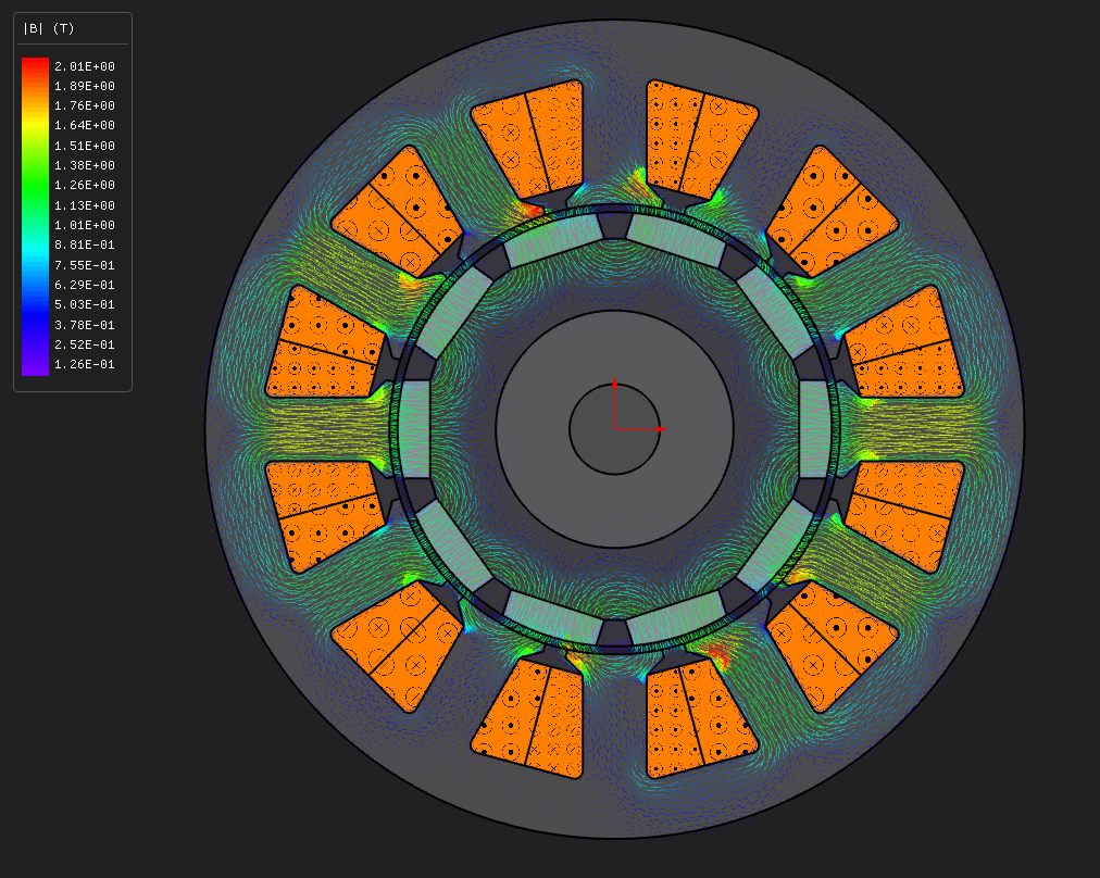
Max B, stator tooth	1.558	T
Mesh	6658 nodes, 12728 elements, P1	—
Wall time, end to end	46	s

Start here. This is a small surface-magnet servo motor — 100 mm across, 50 mm of stack — and it is the quickest thing in the set to open, solve and read. It shows the three results a PMSM is normally judged on: cogging torque, back-EMF and torque under load.

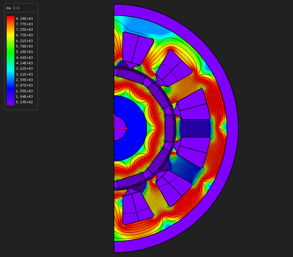
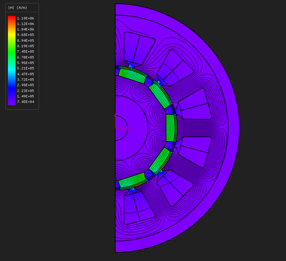
Half the machine is on screen. Twelve slots and ten poles share a factor of two, so six slots and five poles are enough, with an anti-periodic boundary down the two straight edges. The missing half is the same field with the sign reversed, and meshing it would only cost you time.

The design

Layer	Radii (mm)	Set by
shaft bore	5.500	shaftThickness 9 (an 11 mm bore)
rotor shaft	5.5 → 14.5
rotor core	14.5 → 22.5	coreThickness 8
magnet	22.5 → 26.5	PMThickness 4, PMWidth 12 (about 78 % of the pole)
air gap	26.5 → 27.5	airGap 1
stator bore	27.500	ID 55
slot bottom	42.500	slotDepth 15, slotWidth 8
stator OD	50.000	OD 100, back iron 7.5

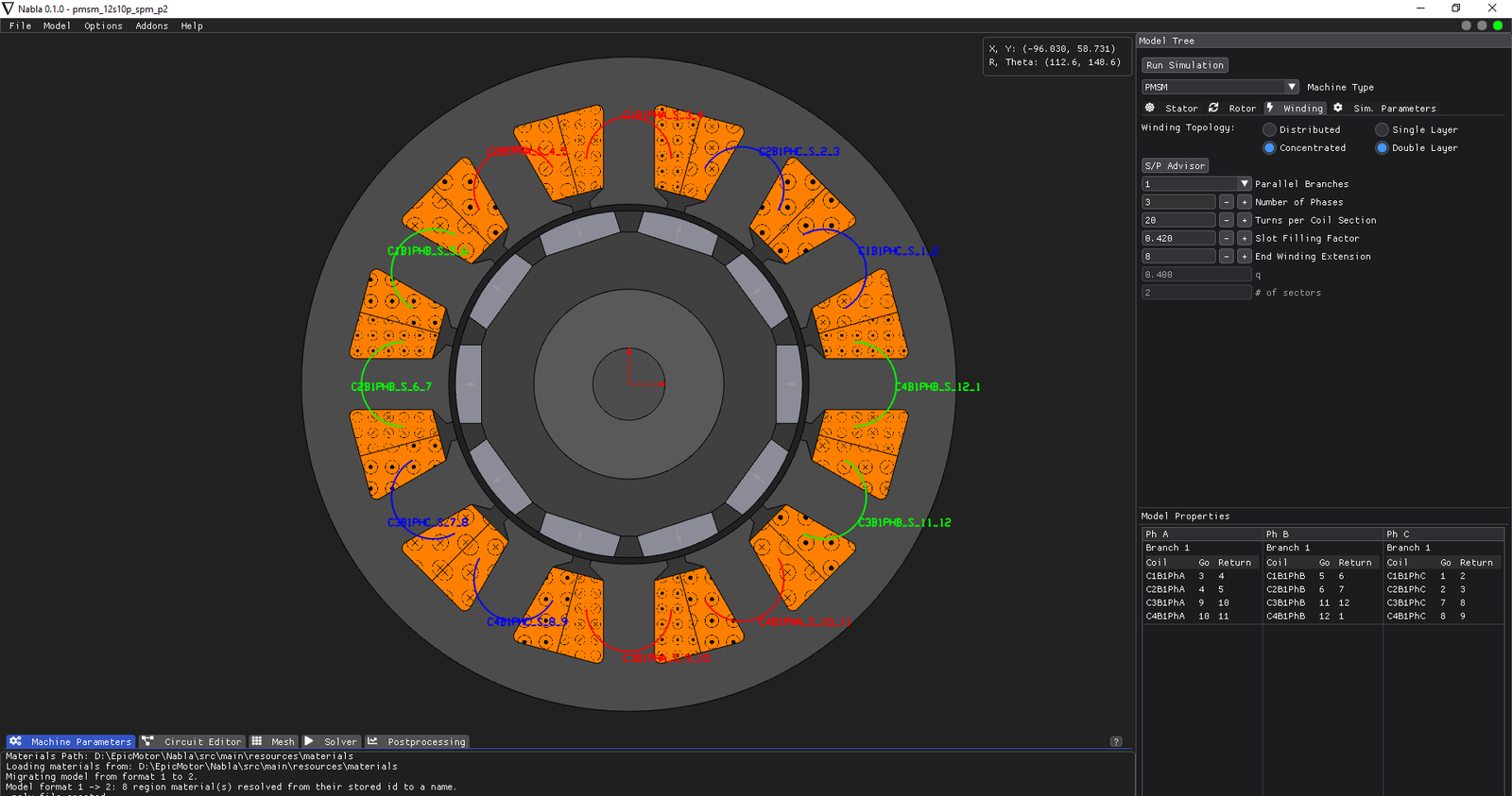
Rectangular teeth, 50 mm axial length, five pole pairs.

Winding and materials

Stator and rotor core	M-19 Steel, nonlinear BH
Rotor shaft	1020_steel
Magnets	N42
Winding	concentrated, double layer, one coil per tooth
Turns per coil	20 (twelve coils, four in series per phase, one parallel branch)
Slot fill	0.42
End winding	8 mm extension, with end-winding resistance and inductance included

Two settings are worth copying if you build your own machine from the template. The template starts with one turn per coil and a placeholder magnet, and neither is usable: turns enter every voltage and every inductance as N², and the placeholder magnet is not a magnet. Set the turns and pick a real magnet material before your first solve.

q = 12 / (10 × 3) = 0.4, which is a fractional-slot concentrated winding, and the winding factor comes out at 0.933.

Operating point

Current	15 A peak, all on the q-axis (I_d = 0)
Speed	2000 rpm, so 166.7 Hz electrical
Window solved	one electrical period, 36 steps
Elements	first order; the --p2 run repeats it at second order
Mesh	0.7 mm maximum

Pure q-axis current is the right choice here because the rotor has no saliency to exploit. See E02 or E04 for machines where the current angle earns its keep.

Running it

Open pmsm_12s10p_spm.nbl and press Solve. The solved field ships with the model, so you can also just open it and look — an expired licence never stops you opening a model or reading results that are already there.

From Python:

python build_pmsm_12s10p_spm.py            # build, solve, render, report
python build_pmsm_12s10p_spm.py --p2       # the same design at second order

The script rebuilds the whole model from nothing, so it is also the readable version of every setting listed above.

What to look at

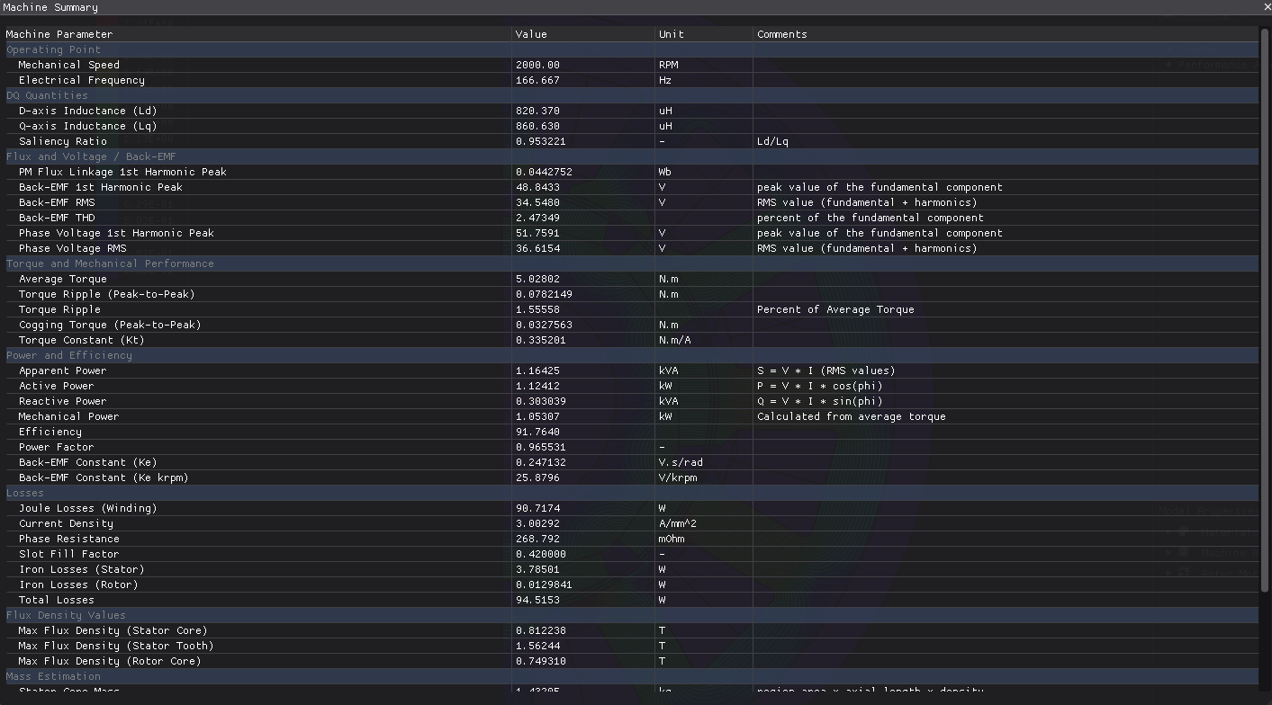
Torque. The average lands near 5 N·m and the ripple is a few per cent. Multiply the torque constant by the q-axis current and you get the same answer, which is what you expect when there is no reluctance term.

L_d and L_q. They come out within a few per cent of each other. That is the signature of a surface-magnet rotor: the magnets are a long magnetic air gap wherever you look, so neither axis is preferred, and there is no reluctance torque to be had.

Back-EMF. Around 35 V RMS at this speed, with about 2 % distortion. The waveform export is in bemf_phaseA.csv if you want to look at the harmonics yourself.

Second-order elements. Run --p2 on the same mesh. Torque rises about 1.5 %, ripple halves and cogging drops by a factor of five. None of that is a design change — it is the first-order discretisation error being removed, and it is a useful calibration of how much to trust a small quantity on a coarse mesh.

How far to trust the cogging number

Cogging for this slot-pole combination is genuinely small, of order 1 % of rated torque, and that puts it near what a mesh of this size can resolve across a 1 mm gap. Refine from 1.5 mm to 0.4 mm and the average torque moves 0.02 %, back-EMF 0.15 % and tooth flux density 0.2 %, while the cogging peak-to-peak wanders between 0.02 and 0.18 N·m.

There is a sampling limit on top of that. This combination has 60 cogging events per mechanical turn, so one electrical period at 36 steps gives you three samples per cogging cycle. That is enough to see the ripple exists, not enough to measure it.

So: torque, back-EMF, flux density and losses are solid at the shipped settings. If cogging is the number your design turns on, refine the mesh, raise the step count, and compare runs against each other rather than quoting a single figure.

Iron loss here uses the machine module's default Steinmetz coefficients rather than coefficients fitted to M-19 data, because no material in the shipped library carries a loss table. E02 and E05 show how to fit your own.

Try this next

• --p2 — second order on the identical mesh, for the comparison described above.
• --mesh-size 0.4 --steps 144 — roughly what the cogging figure needs. About five times the wall time, and it moves the average torque by 0.02 %.
• Widen the magnet. PMWidth from 12 mm toward the 15.4 mm pole pitch gives you more flux and more torque, and a cogging waveform that grows along with it.
• Open the air gap from 1 mm to 1.5 mm and watch the back-EMF, the inductances and the cogging all fall together.

About these numbers

The dimensions are invented but plausible. This is not a copy of a published design and no measurement backs it, so please do not quote it as evidence of accuracy. For that, see the validation dossier, where every case states a reference and a tolerance before it runs.

More from this run