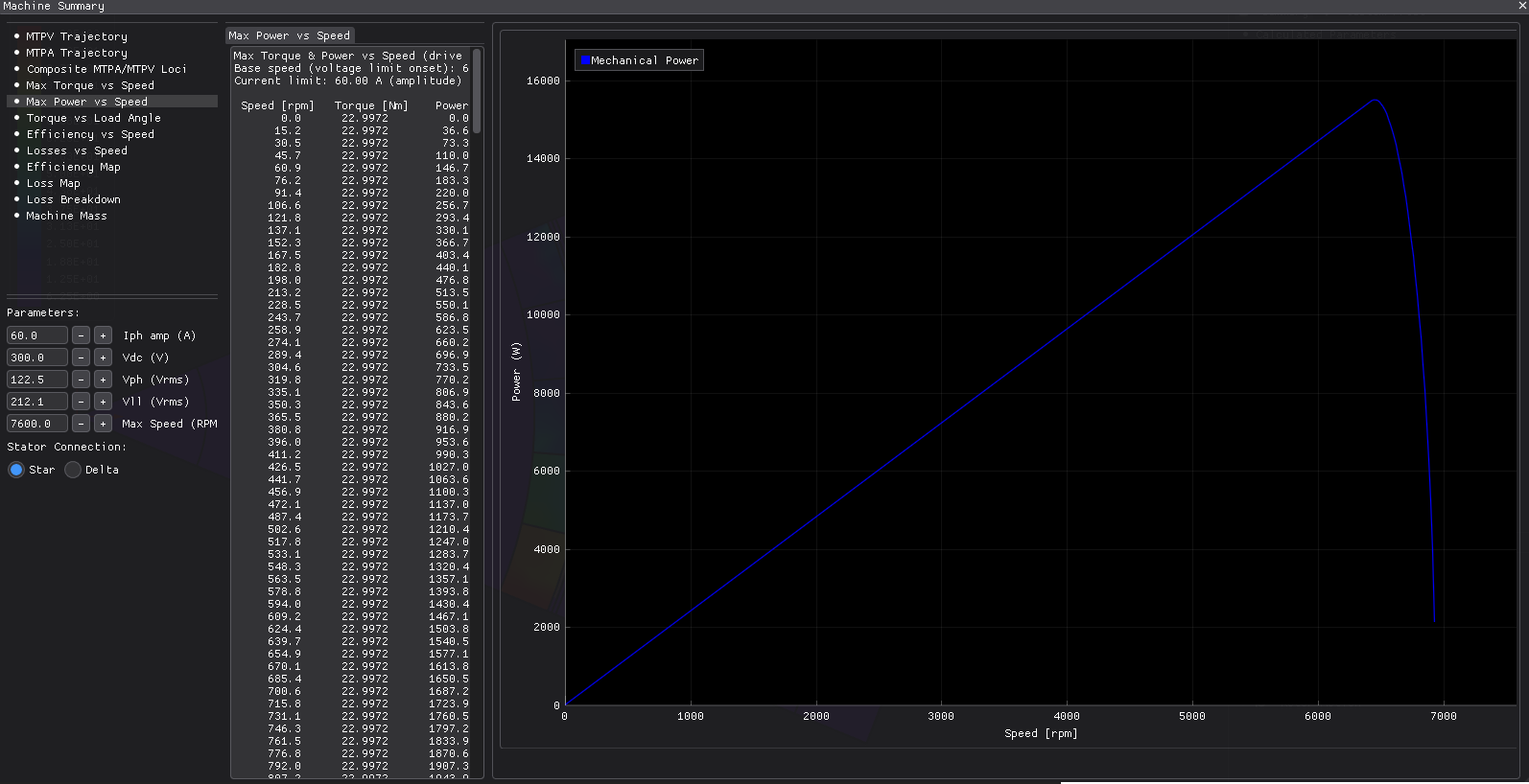
E03 — 48-slot / 8-pole segmented-Halbach PM synchronous machine
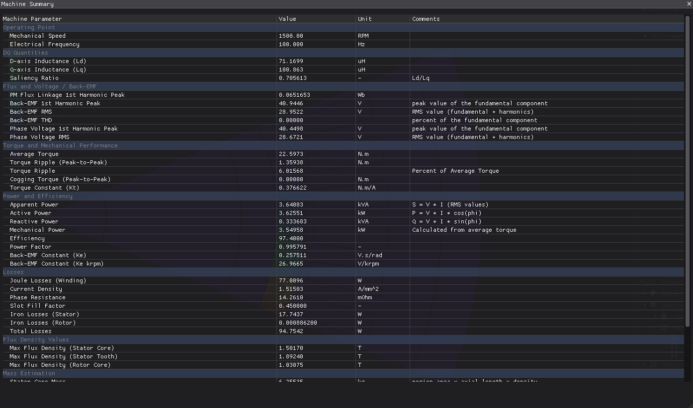
PMSM · Halbach Array · 48 slots / 8 poles · 22.635 N·m at 1500 rpm · 97.4 % efficient · 4256 nodes · 87 s
What you need to run it: the Python API, the Machines module and Core Pro. Opening the model and reading results that are already there never requires a licence. Core Pro covers the multi-slice skew. Without it the machine builds and solves unskewed.
At a glance
| Quantity | Value | Unit |
|---|---|---|
| Speed | 1500 | rpm |
| Electrical frequency | 100.0 | Hz |
| Average torque | 22.635 | N·m |
| Torque ripple | 5.6 | % |
| Back-EMF, RMS | 28.4 | V |
| Mechanical power | 3.555 | kW |
| Efficiency | 97.40 | % |
| Power factor | 0.996 | — |
| Total losses | 94.9 | W |
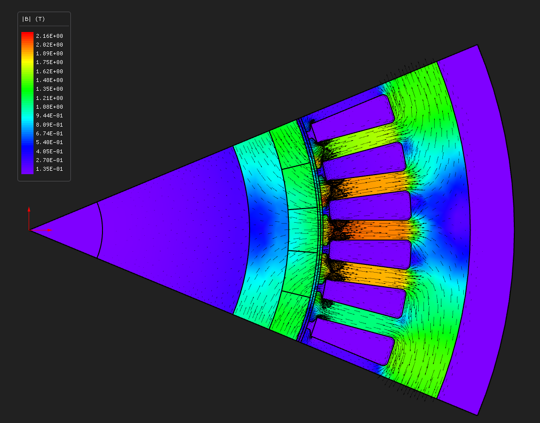
| Max B, stator tooth | 1.965 | T |
| Mesh | 4256 nodes, 8123 elements, P1 | — |
| Wall time, end to end | 87 | s |
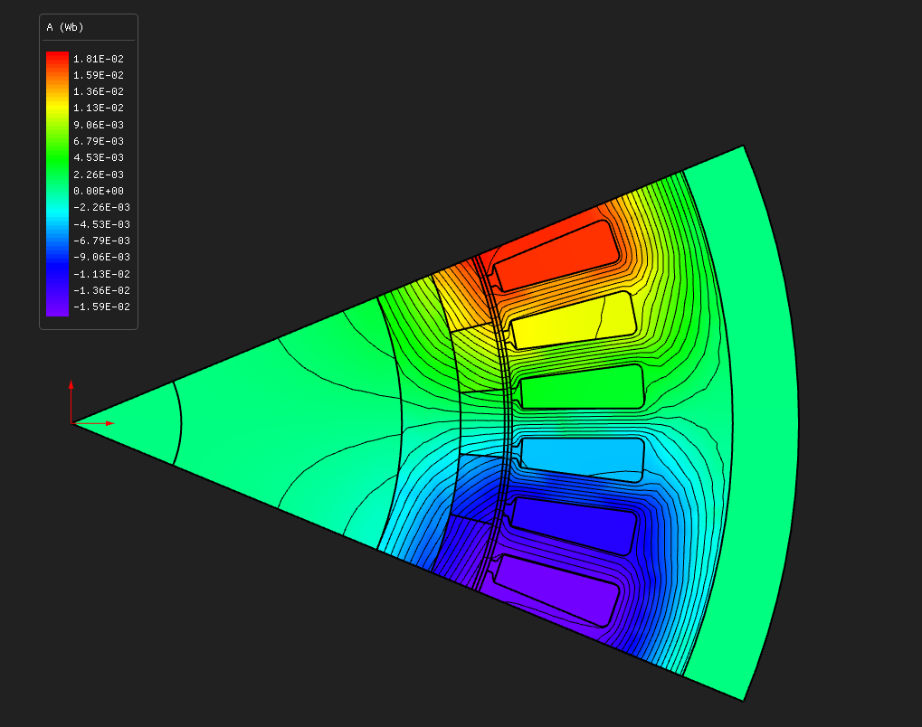
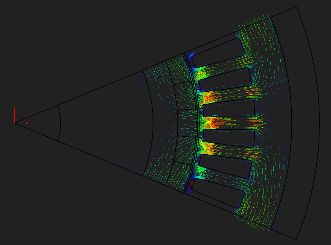
Where the first two examples vary the magnetic circuit, this one varies how the machine is built. Three construction choices are on show, and you can see each of them in the field solution:
- a segmented magnet array — five blocks per pole, each magnetised at a different angle, in the Halbach pattern;
- stator skew, solved as five axially offset copies of the machine at every time step;
- parallel branches — the four coils of a phase wired as four parallel paths.
It also uses the static back-EMF method, which is one magnetostatic solve instead of a no-load sweep, and it has a five-phase variant.
One pole is solved — six slots over 45°, closed anti-periodically.
The design
| Layer | Radii (mm) | Set by |
|---|---|---|
| shaft bore | 15.000 | shaftThickness 30 |
| rotor shaft | 15.0 → 45.0 | |
| rotor back iron | 45.0 → 53.0 | coreThickness 8 |
| magnet array | 53.0 → 59.0 | PMThickness 6, PMSegments 5 per pole |
| air gap | 59.0 → 60.0 | airGap 1 |
| stator bore | 60.000 | ID 120 |
| slot bottom | 78.000 | slotDepth 18, slotWidth 4, slotOpening 0.4 |
| stator OD | 90.000 | OD 180, back iron 12 |
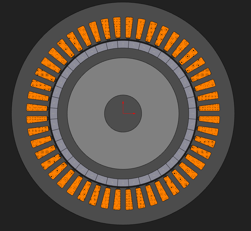
Rectangular teeth, 80 mm axial length, four pole pairs.
How the array is magnetised
PMSegments is the one rotor parameter a Halbach rotor has that a surface-magnet rotor does
not, and PMWidth is one it does not have — a Halbach pole is a continuous arc of blocks with
no gap between magnets to size. Each block is magnetised at
magAngle = (1 − polePairs) · segmentCentreAngle
which is the ideal continuous inner-rotor Halbach law, sampled once per block. The array's own
field is reinforced on the gap side and cancelled towards the shaft. Every block takes the same
magnet material, because the material sets the magnitude and the region sets the direction, so
assigning N42 to all five is right and does not flatten the array.
Use an odd number of segments. With an odd count the d-axis lands on the centre of a block; with an even count it lands on a joint between two. Both work, but the even one is a worse machine, and measurably so — see the sweep below.
Winding and materials
| Stator core and rotor back iron | M-19 Steel, nonlinear BH |
| Rotor shaft | 1020_steel |
| Magnets | N42 |
| Winding | three-phase distributed, single layer, q = 2 |
| Coils | 4 per phase, each spanning two slots on each side |
| Turns per coil section | 12 |
| Parallel branches | 4, one coil per branch |
| Slot fill | 0.45 |
| End winding | 20 mm extension, resistance and inductance included |
Count coils, not slots. A single-layer winding puts one coil side in each slot, which tempts you into "48 slots, so 24 coils, so 8 per phase". The coils here are bigger than that: each spans six slots and occupies twelve slot positions, so the phase has four of them. Four is what the parallel-branch count has to divide, and the model accepts only 1, 2 or 4 — it refuses anything else rather than rounding it. Ask the model for the legal branch counts instead of assuming.
Four branches put one coil in each and split the 60 A phase current into 15 A per conductor. The branch count does not change the torque. It changes terminal voltage and phase resistance, both by the square of the count.
Chording is not available here and cannot be. Shifting one layer of a slot against the other
needs a double-layer winding; a single-layer winding is full pitch by construction, and
setLayerShortening will tell you so and change nothing. E02 is the
chorded machine.
Operating point
| Current | 60 A peak, pure q-axis — a Halbach rotor has nothing to angle into |
| Speed | 1500 rpm, so 100 Hz electrical |
| Skew | 7.5° mechanical, one slot pitch, over 5 slices |
| Back-EMF | static method |
| Window solved | one electrical period, 72 steps |
| Mesh | 1.0 mm maximum, about 4 300 nodes |
Seventy-two steps rather than 36, because the ripple this example is about is the slot harmonic at twelve cycles per electrical period. Six samples per cycle is enough to tell the skewed and unskewed runs apart instead of aliasing one into the other.
Running it
Open pmsm_48s8p_segmented.nbl and press Solve. The solved field is not shipped with this
model, so opening it shows the geometry and the settings until you solve.
From Python:
python build_pmsm_48s8p_segmented.py              # build, solve, render, report
python build_pmsm_48s8p_segmented.py --no-skew    # the same machine, unskewed
python build_pmsm_48s8p_segmented.py --phases 5   # the five-phase variant (40 slots)
python build_pmsm_48s8p_segmented.py --no-solve   # geometry and mesh only
What the skew does
--no-skew runs the identical machine with the twist removed. Mesh, materials and current are
the same.
| skewed (5 slices) | unskewed | change | |
|---|---|---|---|
| Average torque | 22.635 | 23.034 N·m | −1.74 % |
| Torque ripple, peak-to-peak | 1.257 | 6.048 N·m | −79 % |
| Torque ripple | 5.55 % | 26.26 % | |
| Phase voltage, RMS, loaded | 28.694 | 29.242 V | −1.87 % |
| Efficiency | 97.40 % | 97.44 % | −0.05 % |
That is the textbook trade, measured on one machine: a slot pitch of skew takes the ripple down by about four times and costs under 2 % of the torque. The classical skew factor for one slot pitch is 0.9886, so 1.14 % off the fundamental; the measured 1.74 % is a little more because skew averages the harmonics as well.
Read the back-EMF row with care. Several results are identical between the skewed and unskewed runs, and that is not a fault in the comparison. The static back-EMF solve and the inductance solves are single magnetostatic solves that do not carry the slice offset, and the flux-density and loss figures are read off one slice. So:
- the reported open-circuit back-EMF is the unskewed value — multiply by 0.9886 for the skewed machine;
- loaded phase voltage, torque, power, K_t and K_e do carry the skew, because they come from the skewed transient;
- maximum flux density and iron loss describe an unskewed cross-section either way.
How many slices, and what the ripple figure really is
--slices sets how finely the twist is discretised, and the two things it moves behave very
differently. Everything else held:
| slices | T_avg (N·m) | torque ripple | ripple × slices |
|---|---|---|---|
| 1 (unskewed) | 23.034 | 26.26 % | 26.3 |
| 3 | 22.510 | 10.27 % | 30.8 |
| 5 (shipped) | 22.635 | 5.55 % | 27.8 |
| 9 | 22.699 | 3.38 % | 30.4 |
| 15 | 22.726 | 2.36 % | 35.4 |
The average torque converges — the steps are halving, so the continuous-skew answer is near 22.75 N·m and five slices sits about half a per cent below it. The ripple does not converge. It falls roughly as 1/slices right across the range, which is what a quantity looks like when it has not settled at all.
That is the model behaving as it must: N discrete slices cancel the slot harmonic only as far as N shifted copies of it sum to zero, and the residual keeps shrinking as you add slices.
What to take from it:
- 5.55 % is a slice-count-limited number, not this machine's torque ripple. Quote it with the slice count attached. The real continuously skewed machine ripples less than any row here.
- The comparison that does mean something is skewed against unskewed at the same settings, 26.3 % against 5.55 %, because both are the same discretisation of the same quantity.
- If a decision turns on the ripple, run the slice sweep rather than trusting one number.
Average torque, voltages and powers are converged to a few tenths of a per cent by five slices.
What the segmentation does
The same machine at one, two, three, five and seven segments, everything else held:
| PMSegments | T_avg (N·m) | ripple | bEMF RMS (V) | B in rotor back iron (T) |
|---|---|---|---|---|
| 1 (a plain radial ring) | 24.65 | 13.2 % | 30.94 | 1.459 |
| 2 (even — d-axis on a joint) | 21.62 | 18.2 % | 27.28 | 0.860 |
| 3 | 22.43 | 8.5 % | 28.06 | 1.112 |
| 5 (shipped) | 22.63 | 5.6 % | 28.39 | 1.030 |
| 7 | 22.70 | 1.1 % | 28.57 | 1.013 |
Read that honestly, because it is not the usual Halbach sales pitch. One block filling the pole arc — the array collapsed into a plain magnet ring — gives the most torque and the most back-EMF of the lot. What segmentation buys on this machine is the other two columns: ripple falls steadily with the odd segment count, and the rotor back iron carries a third less flux at the same thickness.
The reason is array thickness against pole pitch. Halbach focusing needs a thick array, and 6 mm of magnet against a 44 mm pole pitch is about 0.14 — far too thin, so the tangentially magnetised blocks spend themselves shielding the shaft instead of feeding the gap. Take the array to 14 mm and the ordering flips:
| PMThickness | PMSegments | T_avg (N·m) | bEMF RMS (V) | B in rotor back iron (T) |
|---|---|---|---|---|
| 6 mm | 1 | 24.65 | 30.94 | 1.459 |
| 6 mm | 5 | 22.63 | 28.39 | 1.030 |
| 14 mm | 1 | 26.11 | 32.71 | 1.461 |
| 14 mm | 5 | 26.32 | 33.13 | 0.640 |
This model keeps 6 mm. A 14 mm N42 annulus on a 118 mm rotor is a lot of magnet and it pushes the teeth past 2 T, and the point here is to show what the parameter does rather than to pick the flattering case.
The saliency that is not rotor saliency
The summary reports L_q / L_d = 1.415 for a rotor that is magnetically uniform — magnet everywhere, only the direction varying — and therefore has no rotor saliency at all. The ratio is real, and it lives in the stator, not the rotor. The magnets alone already drive the teeth to about 1.96 T; the inductance stages measure each axis with a small test current on top of that state, so the d-axis increment pushes further into saturation and moves little flux while the q-axis path stays permeable.
If you want to see it directly, run the same model with nonlinear materials switched off and the ratio comes back to 0.999. That run is unphysical in every other respect — it reports 7 T in the teeth — but it settles this one question.
The five-phase variant
--phases 5 is not the same stator, and two things have to change with it.
The slot count. A distributed winding is laid out from q = slots / (2 · poles · phases), and the layout only exists when q is an integer. Forty-eight slots over eight poles and five phases gives 1.2, and the builder then lays out no winding at all — you get coil regions with no phases, a model that meshes and solves and then falls over in post-processing. So the variant uses 40 slots, q = 1, on the same bore and the same rotor. The slot pitch becomes 9°, and the skew follows it.
The excitation. Setting an operating point as I_d and I_q is a three-phase construction. On a five-phase machine that setting is ignored and every phase carries zero current, which converges perfectly happily into a picture of an unexcited machine. The GUI closes that door by disabling Id/Iq definition outside three phases; from a script, set the phase currents yourself.
And the phase angles are not simply 360/m apart. Coils are laid into slots by phase index and the current direction of every odd-indexed phase is flipped, which is the classical phase-belt trick — the same one that turns three belts at 0, 60 and 120 electrical degrees into a balanced set at 0, 240 and 120. For the 40-slot five-phase stator that puts the phases at 0, 216, 72, 288 and 144 degrees: the right five belts, visited in the order A, C, E, B, D. Drive them at −k·72° instead and you excite a standing wave rather than a rotating one. It solves, it converges, the teeth carry 1.87 T, and the average torque comes out at 0.006 N·m with 58 000 % ripple.
Try this next
--no-skewand compare against the shipped run, as in the table above.--slices 9or15to watch the ripple keep falling and the average torque stop moving.PMSegments 1for the plain magnet ring, then 3 and 7, to reproduce the segmentation sweep on your own machine.PMThickness6 → 14 mm to see the Halbach effect actually arrive, and to watch the teeth saturate as it does.
About these numbers
The dimensions are invented but plausible. This is not a copy of a published design and no measurement backs it, so please do not quote it as evidence of accuracy. For that, see the validation dossier.
More from this run