E06 — 24-slot / 8-pole interior-PM outrunner on a drawn rotor, 120 mm across

← Back to the examples

What you need to run it: the Python API and the Machines module. Opening the model and reading results that are already there never requires a licence.

At a glance

Quantity	Value	Unit
Speed	3000	rpm
Electrical frequency	200.0	Hz
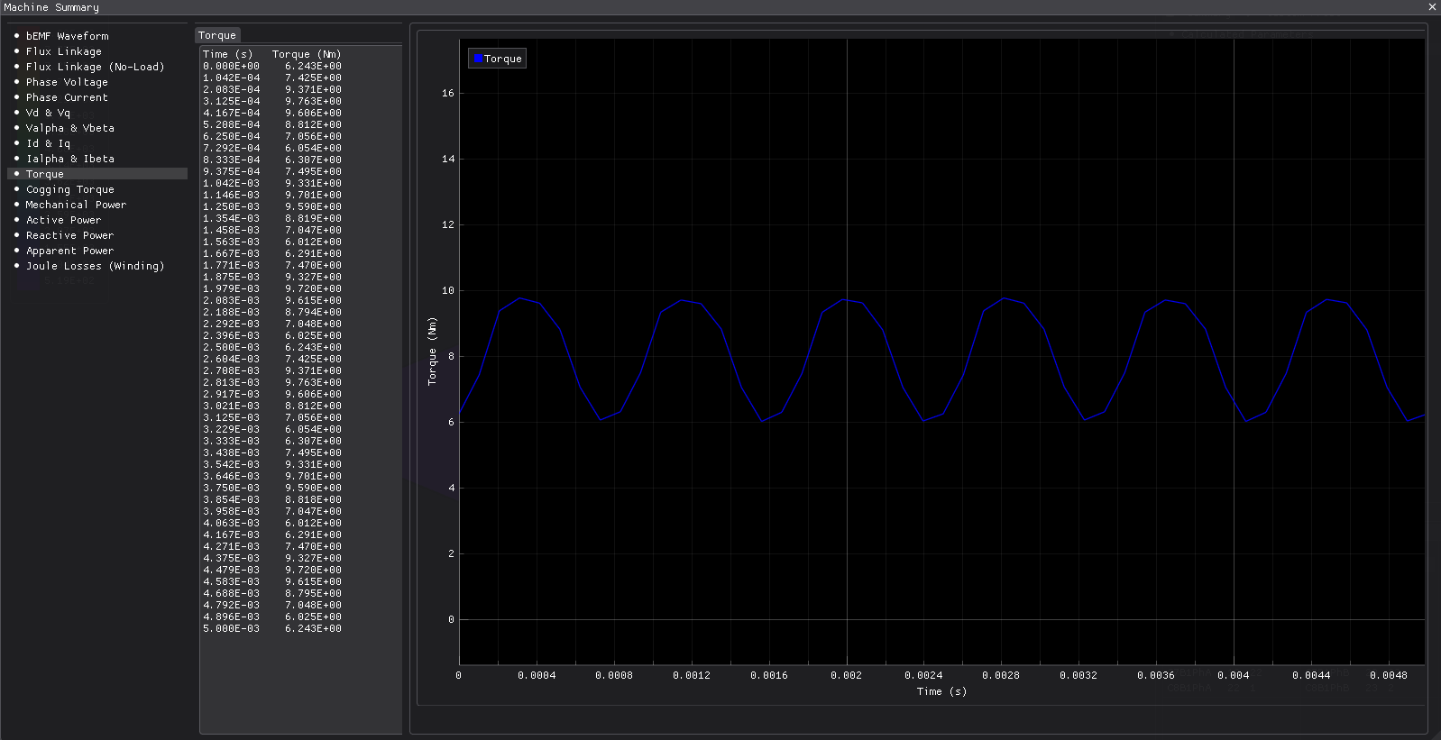
Average torque	8.038	N·m
Torque ripple	46.7	%
Cogging torque, peak-peak	0.584	N·m
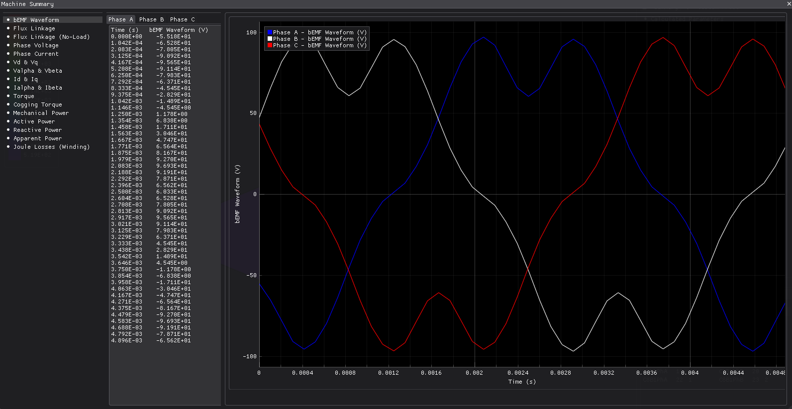
Back-EMF, RMS	66.0	V
Mechanical power	2.525	kW
Efficiency	94.53	%
Power factor	0.985	—
Total losses	146.3	W
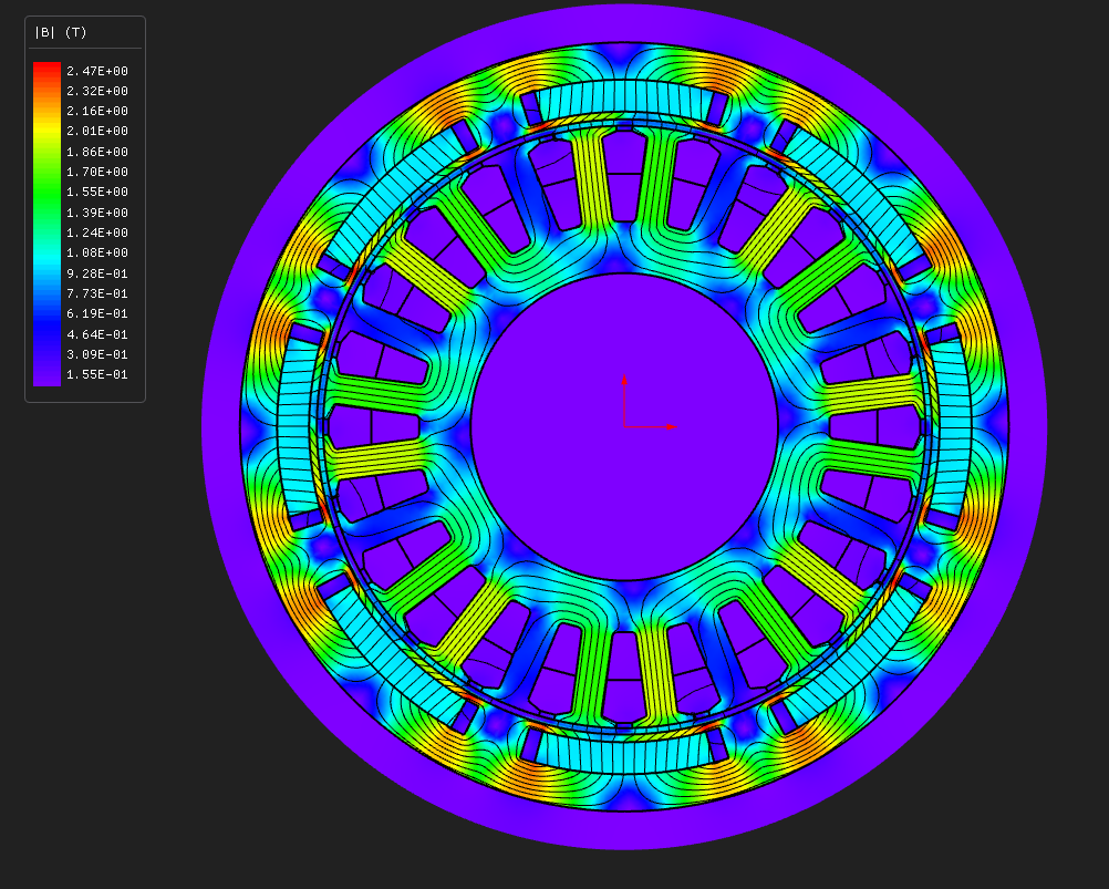
Max B, stator tooth	1.870	T
Mesh	3585 nodes, 6895 elements, P1	—
Wall time, end to end	41	s

A 2.5 kW direct-drive outer-rotor motor with buried magnets. It combines the two harder routes in one model: an outrunner, and a rotor you draw yourself as a DXF.

The difference from E04 is the shape of the domain you are drawing into. An inner rotor is a disc — a triangular sector from the machine axis out to the rotor surface, with the gap on the outside. An outrunner's rotor is the radial inverse: an annular band, with the gap-facing surface on the inside, the rotor outside diameter on the outside, and nothing at the centre but the stator. Everything below follows from that inversion.

One pole is solved — three slots over 45°, closed anti-periodically.

The design

Worked outward from the central bore, which on an outrunner belongs to the stator:

Layer	Radii (mm)	Set by
bore	24.000	derived: slot bottom − stator coreThickness
slot bottom	32.000	stator coreThickness 8
stator iron OD	47.000	slotDepth 15, slotWidth 7, so stator OD 94
air gap	47.0 → 48.0	airGap 1.0, no sleeve
rotor band	48.0 → 60.0	rotor RotorThickness 12
… pole-shoe bridge	48.0 → 49.2	drawn: bridge 1.2
… magnet and barriers	49.2 → 54.2	drawn: cavityDepth 5, magnet ±15°, cavity ±17.5°
… rotor back iron	54.2 → 60.0	what the band has left, giving 120.0 mm outside

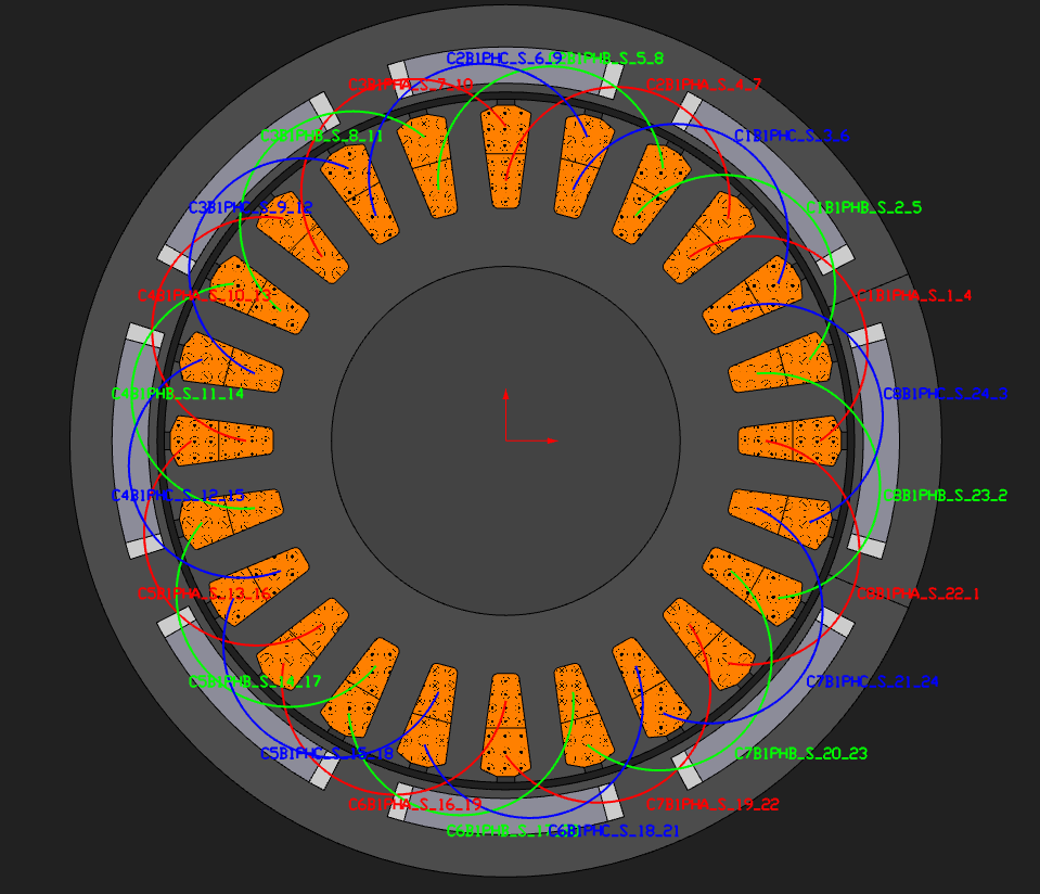
Rectangular teeth, 45 mm axial length, four pole pairs, q = 1, full pitch.

The slot is parallel-sided, so the tooth is narrowest at the slot bottom. At 24 slots the pitch down there is 8.38 mm, and a 7 mm slot leaves a 1.38 mm tooth against 9.30 mm at the tip. That bottom is what sets the peak tooth flux density, and it is the dimension to watch if you widen the slot. A trapezoidal stator is the version of this that keeps the tooth parallel instead of the slot.

The band, and what you may draw in it

A custom rotor takes three parameters: pole pairs, air gap and RotorThickness. Note that RotorThickness is the band's radial depth, not a diameter. Everything inside the band is drawn by you.

The module draws the band's own frame — the inner arc at the gap surface, the outer arc at the rotor OD, the outer air ring, and the two radial seams that carry the periodic pairing — and it does not split any of them where your drawing happens to touch. An entity that ends part-way along one of them makes a T-junction, the polygon description cracks, and a neighbouring region floods across the crack.

That failure is completely silent: the model meshes, the band check passes, the solver converges, the field plot looks normal, and only the flux is wrong.

So every feature here floats inside the band and touches nothing. That is not a coincidence of this design — it is the drawing rule for the annular domain, and it is why the pole shoe has a 1.2 mm bridge under it and the barriers stop 5° short of the pole edge instead of running out to the boundaries. Both are real design numbers anyway.

The script checks the mesh rather than trusting the drawing: every region seed must own elements, and a permeability probe in the back iron must read steel rather than air. Copy that habit into your own models — it is a few seconds and it catches the one failure you cannot see.

The rotor drawing

One cavity per pole, drawn as a polar rectangle: two arcs and two radial walls, split by two more walls into a magnet in the middle and an air barrier at each end. Ten entities, all generated from four numbers. Each arc is emitted already split at every wall that ties into it, so a wall's endpoint is a shared corner rather than a point part-way along a longer entity.

Two dimensions decide the machine:

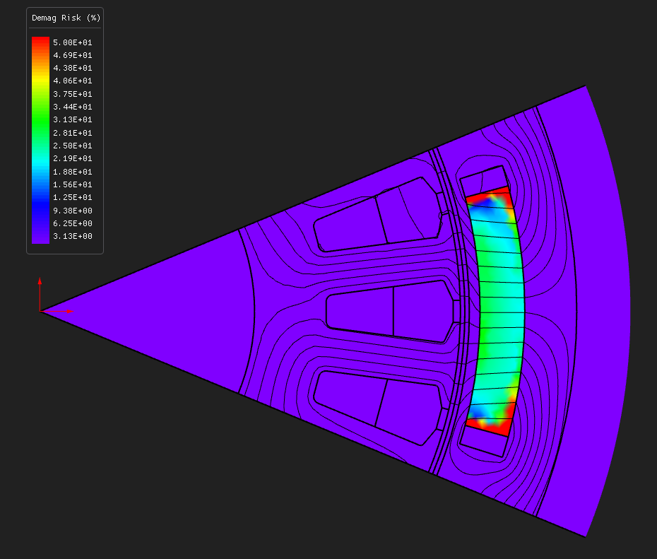
The 1.2 mm bridge between cavity and gap surface is the pole shoe. It is both a useful flux path and the leakage path that short-circuits the magnet. It runs at about 1.18 T on the d-axis here, and a bridge wants to be at saturation — a comfortable bridge is one that is stealing the magnet's flux. This one is only comfortable because the narrow tooth saturates first and holds the whole path back. On a 4 mm slot the same bridge runs at 1.69 T.

The 5° of iron at each pole edge is the q-axis channel. It is what makes a drawn rotor salient, and it is part of where L_q / L_d = 2.23 comes from.

Like E04, the .dxf is an output regenerated on every run, so hand edits are discarded unless you pass --keep-dxf — and even then the region seeds and magnetisation come from the script.

Magnetisation points outward

The magnet is magnetised along the pole axis at 0°, which is radially outward — away from the air gap, because on an outrunner the gap is on the inside. That is the opposite of an inner rotor's north pole.

Nothing about getting it wrong looks wrong. It converges, it draws the same picture, and the only symptom is that the average torque comes out negative. This model was built the other way round first.

Winding and materials

Stator core and rotor lamination	M-19 Steel, nonlinear BH
Magnet	N42SH
Flux barriers	air
Winding	three-phase distributed double layer, q = 1, full pitch
Turns per coil	10, one parallel branch
Slot fill	0.42
End winding	8 mm extension

Iron loss on a region you seeded yourself needs its coefficients. The machine module enables iron loss on the stator core it built and seeds that region's Steinmetz coefficients for you. A region created by a script starts with all three at zero, and the loss terms multiply by them, so switching iron loss on buys you a clean and plausible 0 W. Here the coefficients are copied off the stator core, which is the same steel, and read back from the model rather than written down twice.

With them in place the rotor iron loss comes back at about 2 × 10⁻⁵ W — still zero, but now for the physical reason rather than the arithmetic one. A synchronous machine's rotor iron carries a flux that is nearly DC in the rotor's own frame, so there is no cycle to charge.

Operating point

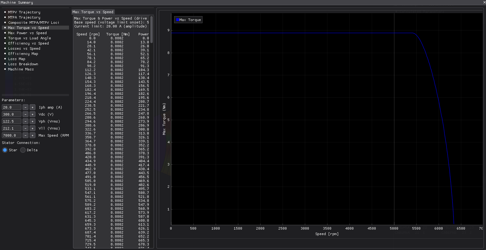
Current	20 A peak at 25° current angle, so I_d = −8.5 A, I_q = 18.1 A
Speed	3000 rpm, so 200 Hz electrical
Window solved	one electrical period, 48 steps
Eddy currents	off; the magnets are treated as insulating
Mesh	1.2 mm default; 0.6 mm in the lamination, 0.9 mm in magnet and barriers

The lamination gets the finer mesh because it carries the 1.2 mm bridge, and a bridge two elements wide is not a bridge.

Running it

Open pmsm_outrunner_custom_rotor.nbl and press Solve. The solved field is not shipped, so opening shows geometry and mesh until you solve.

From Python:

python build_pmsm_outrunner_custom_rotor.py              # build, solve, render, report
python build_pmsm_outrunner_custom_rotor.py --no-solve   # geometry and mesh only
python build_pmsm_outrunner_custom_rotor.py --help       # every flag

About half a minute end to end on a laptop.

What to look at

The torque split. From the solved inductances and magnet flux, the dq model gives 7.69 N·m of magnet torque and 0.46 N·m of reluctance torque against 8.04 N·m solved. The reluctance share is only 5.7 %, even though L_q / L_d is 2.23. This rotor is salient, but it is still a magnet machine, and at 25° of current angle the reluctance term is a garnish. E04's V-pocket rotor gets 33 % from the same split.

Worth noticing where that high ratio comes from: it is L_d collapsing rather than L_q rising — 411 µH here against 797 µH with a 4 mm slot. A saturating stator looks like q-axis saliency, and here it stacks on top of the rotor's own.

Torque ripple is 47 %, and it is the design, not the mesh. One slot per pole per phase means the distribution factor is 1 for every harmonic, and a full-pitch coil cancels none of them, so nothing in the winding suppresses what the pole shape and the slotting produce. Refine the mesh from 1.2 to 0.8 mm and torque, back-EMF, inductance, tooth flux density and iron loss all move by under 0.2 %, while the ripple moves 3 % and the cogging 7 %. The field is converged; the ripple is the machine, and it is the price of the wide slot.

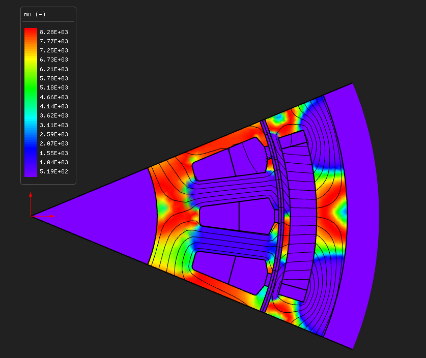
The permeability map (region_map_mu.png) is the quickest check that a drawn rotor came out the way you meant: steel where you wanted steel, air in the barriers, magnet in between.

Try this next

• Widen the barriers. cavityHalfAngle 17.5 → 19.5 narrows the q-axis channel from 5° to 3°: L_q falls, saliency falls with it, and the reluctance share shrinks. Keep it under 22.5° or the cavity reaches the sector seam and you hit the T-junction problem above.
• Thin the bridge. bridge 1.2 → 0.7 leaks less magnet flux, so back-EMF and torque both rise and the bridge saturates harder. Going the other way, to 2.0 mm, is the cheap demonstration of what a bridge costs you.
• Sweep the current angle from 0° to 45° to trace this rotor's MTPA curve.
• Narrow the slot. slotWidth 7 → 4 widens the tooth bottom from 1.38 to 4.38 mm, brings the tooth off saturation and roughly doubles L_d — which is the direct way to see how much of the saliency was the stator rather than the rotor.

About these numbers

The dimensions are invented but plausible. A 120 mm direct-drive outer-rotor motor is a class of machine, not a particular product, and no measurement backs it. For accuracy claims, see the validation dossier.

More from this run