Eddy-current brake — drag against speed, through a sliding band
Non-machine · Planar transient with linear motion · 8 poles · peak drag 864 N at 10 m/s · power balance within 1.75 % · 3393 nodes · 1 min 22 s
What you need to run it: the Python API (Automation) only. One motion zone, the sliding band and eddy currents are all free-tier capabilities, and the mesh is well under the free node budget.
What this one is for
This is the motion demo of the set, and the only example whose eddy currents are produced by movement rather than by an AC source. Nothing in the model carries an impressed current. The source is a permanent magnet, and every ampere in the rail is there because the rail is sliding.
It is therefore the shortest complete demonstration of Nabla's sliding band on a device with no rotor, no windings and no machine module — and the three rules that make a band work are each written out at the site in the script where they apply.
At a glance
| Quantity | Value | Unit |
|---|---|---|
| Magnet array | one per 25 mm pole pitch, 10 mm thick, alternating, N42 | — |
| Back-iron | 10 mm, linear, μr = 2000 | — |
| Airgap, magnet face to rail | 3 | mm |
| Rail | 6 thick × 50 wide, aluminium, σ = 3.5e7 S/m | mm |
| Brake | 8 poles (the model is one pole pitch) | — |
| Peak drag | 864 at 10 m/s | N |
| Drag at 0.5 / 20 / 60 m/s | 94.0 / 774.0 / 560.2 | N |
| Power balance, |F|v vs Joule loss | 1.75 worst (tolerance 4) | % |
| Low-speed slope vs closed form | 23.51 vs 23.54 N/(m/s), 0.1 | % apart |
| Mesh | 3393 nodes, P1 | — |
| Wall time, 11 runs / 1228 steps | 1 min 22 | s |
The model is one pole pitch
The magnet array and the rail are both uniform along the direction of travel, so the device is periodic with the magnet pitch — and anti-periodic over one of them, because the next magnet is the same magnet upside down. The model is therefore one pole pitch wide, with parallel anti-periodic sides and an anti-periodic linear sliding band, and it stands for an infinitely long brake. That is what makes the whole eleven-point sweep fit in under a minute and a half on 3393 nodes.
The back-iron is linear on purpose. This example is about eddy currents, not about a BH table, and at this magnet loading the iron never approaches its knee; turning saturation on would make every step a Newton loop and change nothing worth reporting.
The sliding band — three rules
This is the part worth copying, and each rule has bitten real models before.
- The speed is in model length units per time unit. A linear motion profile's value is millimetres per second on a millimetre model — the peer of a circular profile's degrees per second. Getting it wrong gives a perfectly converged solution at a thousandth of the intended speed.
- The strip between the band's two rings must not be meshed. The band's job is to stitch the moving ring to the stationary one at each step, and it can only do that if the two rings are genuinely separate boundaries of the mesh. Here they sit 1 mm apart inside the 3 mm airgap and the strip between them is a hole, never a region. Nabla's rule M16 refuses a mesh that fills it — but the failure M16 prevents is silent at zero displacement, so a standstill check passes and the moving solution bleeds away instead. Do not write the script so that M16 has to catch you.
- The motion zone must end between the two rings. The band decides what the solver couples; the zone decides what post-processing translates into the lab frame. A zone drawn past its own ring translates stationary air at probe and render time while the force stays plausible — a defect that hides.
The window sides are drawn as two runs for the same reason: nothing may cross the band strip, so each side is interrupted there, and every interval ends exactly where a layer does so that no side segment carries a T-junction — which is what a periodic marker gets lost to.
The result
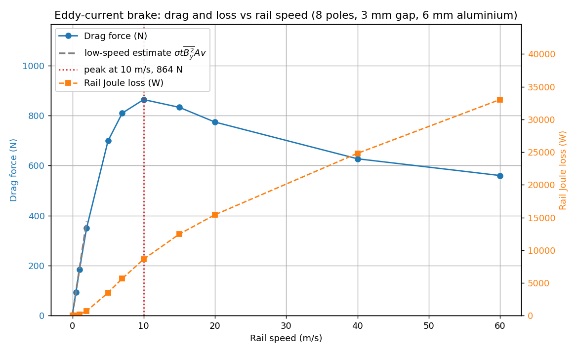
  speed    drag/pitch   drag(8 poles)     Joule       |F|*v    balance
    0.5 m/s     11.75 N        94.0 N         5.8 W         5.9 W     0.92%
    1.0 m/s     23.02 N       184.2 N        22.9 W        23.0 W     0.42%
    2.0 m/s     43.84 N       350.7 N        87.5 W        87.7 W     0.19%
    5.0 m/s     87.35 N       698.8 N       436.4 W       436.8 W     0.08%
    7.0 m/s    101.23 N       809.8 N       707.9 W       708.6 W     0.10%
   10.0 m/s    107.99 N       863.9 N      1077.6 W      1079.9 W     0.21%
   15.0 m/s    104.12 N       833.0 N      1557.1 W      1561.8 W     0.30%
   20.0 m/s     96.75 N       774.0 N      1927.0 W      1935.0 W     0.41%
   40.0 m/s     78.40 N       627.2 N      3101.2 W      3135.9 W     1.12%
   60.0 m/s     70.02 N       560.2 N      4128.9 W      4201.4 W     1.75%
The shape is the physics. Drag rises linearly with speed while
the induced field is negligible, peaks at 10 m/s at 864 N, and falls
beyond it as the eddy currents begin to shield the rail from the magnets. A brake
designed on the rising branch and operated past the peak brakes less the
faster it goes, which is why the peak is the number that matters. The dissipated
power keeps climbing throughout — it is |F|v, and the force falls
more slowly than the speed rises.
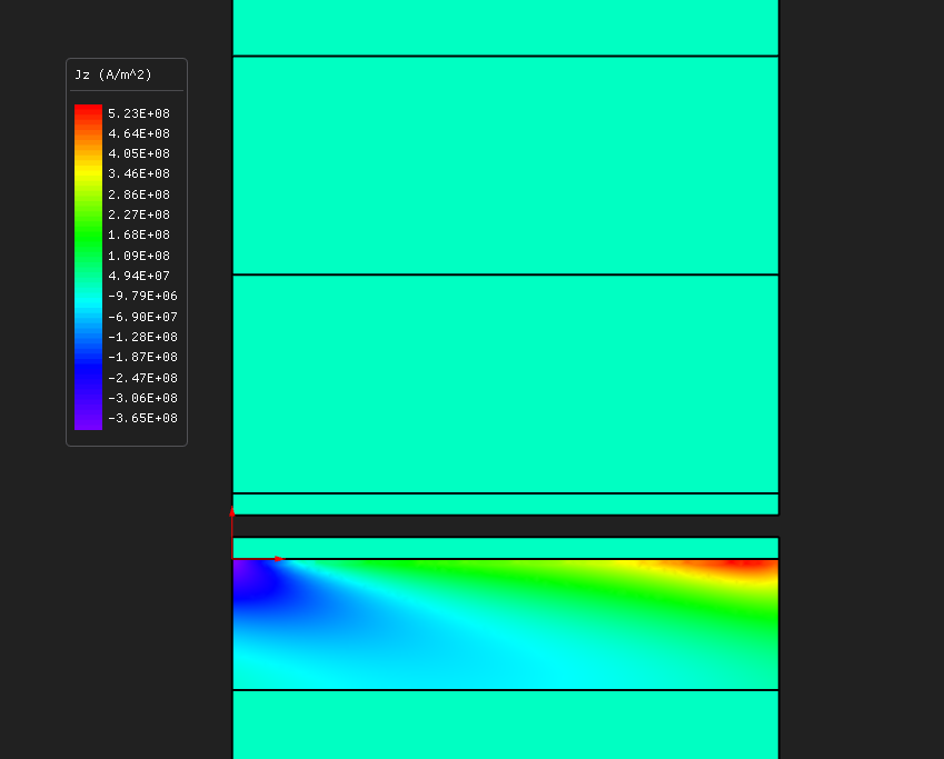
That is the drag itself: a current sheet in the rail, lagging behind the magnet it was induced by. The gap across the middle of the picture is the band strip — it is a hole, so there is nothing there to draw.
The checks
Power balance — the tight anchor. |F|v against
the rail's Joule loss, required within 4 %, worst case 1.75 %. These
are two entirely independent post-processing paths on the same solution — a
Maxwell-stress contour integral on the band, and a volume integral of
J²/σ over the rail — and nothing else in the model
dissipates, so they have to agree.
Low-speed slope — the analytic anchor. With the induced
field neglected, J = σvBy, so
dF/dv = σ·t·⟨By²⟩·A.
Measuring ⟨By²⟩ inside the rail on the
stationary solution gives 0.0897 T², predicting 23.54 N/(m/s)
per pole pitch against 23.51 measured at 0.5 m/s — 0.1 %
apart. The tolerance is deliberately loose at 25 %, because the closed form ignores
the induced field entirely; the agreement being this good is a property of
this operating point, not a promise.
The zero-speed point is the uncertainty band on the whole curve. No motion means no eddy currents — the Joule loss comes back at 4.8e-30 W — so the drag there is exactly zero. What the force integral reads instead, 0.378 N, is its own noise floor, and it reads on every other point too: 0.35 % of the peak, but 3.2 % of the 0.5 m/s point. The example prints it rather than subtracting it. It moved from 0.132 N to 0.378 N on refinement, so it is mesh noise and not a physical offset.
Two mesh and window decisions, measured rather than assumed
How long a run has to be. Each speed runs for the longer of three pole pitches of travel and five of the rail's own diffusion times (1.6 ms for 6 mm of aluminium). At 0.5 m/s the travel window binds; at 20 m/s three pitches is only 3.75 ms, barely two diffusion times, and the drag would be averaged over a startup that has not finished. Measured: at 20 m/s the power balance closes to 6.1 % on a 3-pitch window and 2.0 % on a 6-pitch one, while doubling the step count on the 3-pitch window moves it by 0.08 %. The error was settling, not time discretization, and the fix is a longer run rather than a finer one.
The rail mesh is the one number that is not comfort. The skin depth at the top swept speed is 1.74 mm inside a 6 mm rail, so the rail needs several elements through depth. Measured at 60 m/s:
| Rail mesh | Nodes | Joule loss | |F|·v | Power balance |
|---|---|---|---|---|
| 0.15 mm² | 1758 | 3950 W | 4208 W | 6.55 % |
| 0.05 mm² | 3393 | 4129 W | 4201 W | 1.75 % |
It is the Joule integral that moves, not the force contour: an
under-resolved skin layer under-reads J²/σ. Halving the time
step at either mesh changes the balance by 0.01 %.
Caveats
- The 40 and 60 m/s points carry about 3 % of Backward-Euler time-discretization error in the absolute drag. The power balance cannot see it, because both sides move together. Those two points exist to show the falling branch; the interesting range, up to 20 m/s, is converged.
- Both irons are linear, so this example says nothing about a saturating back-iron. A back-iron thin enough to saturate is a different — and worse — device.
Running it
python eddy_current_brake.py            # build, solve the sweep, check, plot
python eddy_current_brake.py --coarse   # every mesh area x4, 28 s
python eddy_current_brake.py --no-solve # geometry and mesh only
--coarse reproduces the whole curve to within 2 % and is judged
against a looser power-balance bar, because its rail cannot resolve the skin depth at
the top two speeds — and the run says so.
Try this next
- The airgap is the single biggest lever on the drag, and it enters roughly squared.
- Rail thickness and conductivity set the low-speed slope and move the peak: more of either means more drag at low speed and an earlier peak.
- Pole pitch — a longer pitch pushes the peak to a higher speed, because the excitation frequency a given speed produces is lower.
- Make it rotary. A disc between magnet poles is the same example with a circular motion and arc band boundary conditions instead of the line pair — and the speed then goes in degrees per second.
About these numbers
This is a demonstration brake, not a product. Every figure on this page came out of the run described here at the settings the script ships with. For accuracy against a stated reference and tolerance, the validation dossier is where that question belongs.