Gauss gun — a single-stage coilgun from force map to muzzle velocity

← Back to the examples

What you need to run it: the Python API (Automation) and nothing else — a static or transient P1 run, planar or axisymmetric, is Core. The script checks up front and exits cleanly with a message rather than failing at the solver.

What this one is for

This is the largest of the non-machine examples: one script that uses the static solver, the transient solver, an external circuit and a nonlinear BH curve on the same device, and then does something with the numbers. If you want to see how the pieces of the API fit together on a real design question, this is the one that puts all of them in the same file.

It is also the example that is most explicit about a limit. Nabla's motion is prescribed: you give it a speed profile and it gives you a field solution. A real gun's velocity is an output of the force being computed, so a single self-consistent field-plus-mechanics solve is not something this solver — or most 2D FEM solvers — does. Rather than imply otherwise, this example does what an engineer actually does: measure the force with FEM, integrate the mechanics separately, and then measure the error of having done so.

At a glance

Quantity	Value	Unit
Barrel	ID 8, OD 10, 140 long, non-magnetic	mm
Drive coil	ID 10, OD 20, 25 long, N = 300	mm
Projectile	Ø7.5 × 20, 6.95 g, 1020 steel (BH), σ = 5.9e6 S/m	—
Drive	300 V switched DC through 1.7 Ω total	—
Peak attractive force at 100 A	85.3	N
F(z) zero crossing	+0.22 (coil centre is 0)	mm
Eggshell vs virtual work, 10 A / 100 A / 200 A	7.0 / 51 / 53	% apart
F/I² retained from 10 A to 200 A	13	%
Coil inductance at the launch start	0.513	mH
Peak coil current in the pulse	175.5	A
Transient force vs the quasi-static surface	11.2 of the peak	%
Optimum turn-off / muzzle velocity	1.50 ms / 25.1	m/s
Energy efficiency at the optimum	3.5 (67.6 J in, 2.2 J out)	%
Energy audit residual	0.69 (tolerance 5)	%
Wall time, all three stages	3 min 15	s

Stage 1 — the force map

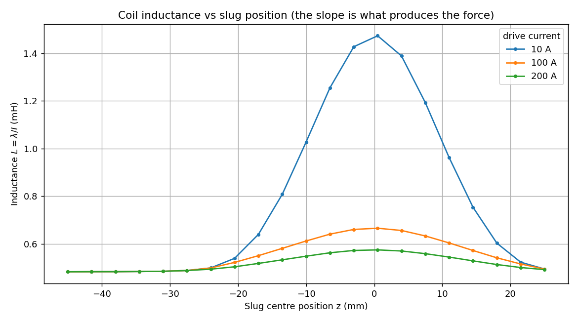
The slug is parked at 21 axial positions from 45 mm behind the coil to 25 mm past its centre, remeshed at every point and solved at three currents — 63 static solves. Two checks fall straight out, and both are physics rather than fitted tolerances.

F(z) crosses zero at the coil centre, measured here at z = +0.2 mm. That crossing is the entire design problem of a coilgun: past the centre, the same current pulls the slug back.

The virtual-work identity holds only at the lowest current. F = ½I²·dL/dz matches the eggshell force to 7 % at 10 A and is off by more than 50 % at 100 A and 200 A — because that identity is a linear one and this slug is saturated. Both numbers are printed rather than only the flattering one. The saturation is also why the map is taken at three currents at all: between 10 A and 200 A, F/i² retains only about a tenth of its low-current value, so scaling one map by i² would be wrong by an order of magnitude, and stage 3 interpolates across currents instead.

Stage 2 — the real drive, and the error it measures

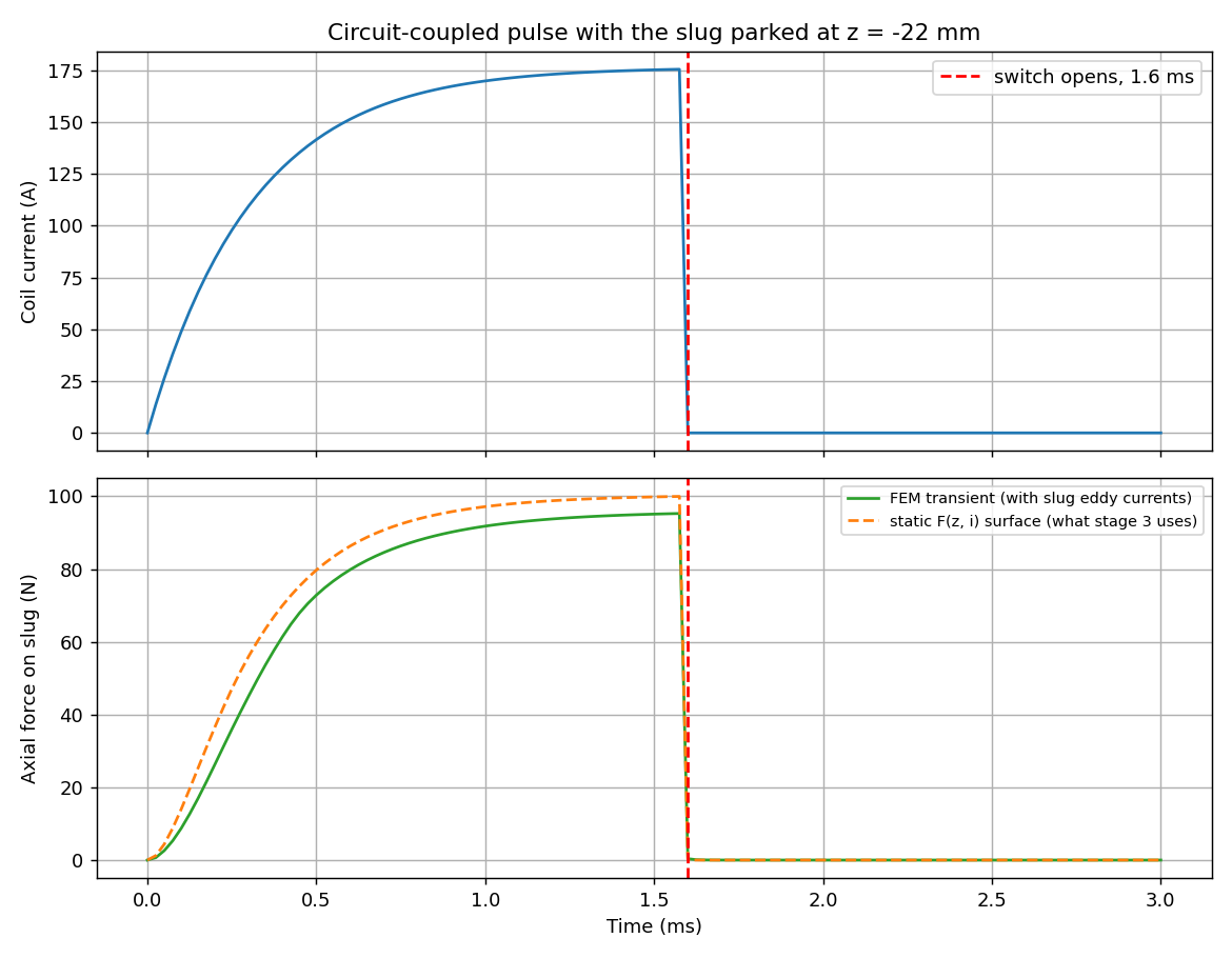
The slug is parked at the launch start position and the actual netlist is solved: a 300 V DC supply, a switch that opens at t_off, 0.5 Ω of series resistance and the coil's own 1.2 Ω winding resistance — with saturation on, the circuit solver on, and eddy currents on. The slug is solid steel, and the currents induced in it oppose the pull.

That is what makes stage 3 believable: the transient force history is compared against the quasi-static surface stage 1 measured, and the departure is 11.2 % of the peak. The approximation the launch model rests on has a printed error bar instead of an assumption.

Why not a charged capacitor? The natural coilgun drive is a capacitor discharge, and a C element exists — but the solver's capacitors start at zero volts and there is no initial-condition field, so a source plus a capacitor charges rather than discharging. This example uses a switched DC supply through a series resistance, which is a real drive (a MOSFET-switched bench supply) and is honest about being one. A true capacitor discharge can be reproduced by putting the analytic RLC ring-down on a "Custom" voltage source, and the script shows the four lines that does.

Stage 3 — flying the slug

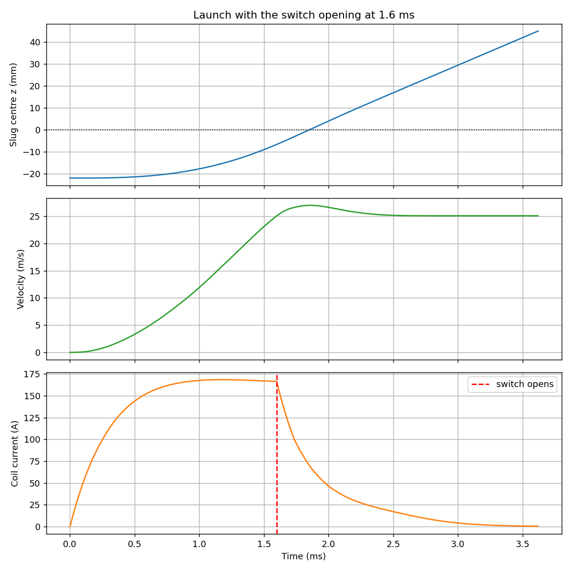
Pure Python, no solver: RK4 on

m dv/dt = F(z, i)                        F from the measured surface
dz/dt   = v
(dlambda/di) di/dt = V - i R - v dlambda/dz

Two decisions in there are physics rather than bookkeeping. The current equation uses the incremental inductance dλ/di and the motional term v·dλ/dz, not L = λ/i and dL/dz — on a saturating device those differ by nearly a factor of two, and the incremental pair is what the circuit actually sees. And the motional back-EMF term is the coupling: it is what takes energy out of the supply and puts it into the slug. Dropping it is the classic coilgun-model error, and it makes the gun look better than it is.

The map covers 45 mm behind to 25 mm past the coil; beyond that the device's own mirror symmetry about the coil centre supplies the rest exactly, so the slug can be flown out to the muzzle. The stage closes with an energy audit — supply energy in against I²R, slug kinetic energy and the energy left in the field — which closes to 0.69 %.

The figure that pays for the whole example

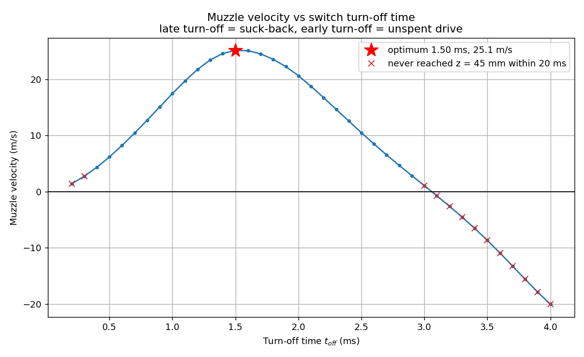
Muzzle velocity against turn-off time. There is a clear optimum at 1.50 ms giving 25.1 m/s, with the suck-back penalty on the late side — leave the coil on and it pulls the departing slug backwards — and the unspent-drive penalty on the early side. Getting the timing wrong by 20 % costs 13.4 % of the muzzle velocity late and 6.3 % early.

Energy efficiency at the optimum is 3.5 %: 67.6 J in, 2.2 J out. A single-stage coilgun is a few percent, and this one is no exception.

The stage that is not here

The obvious fourth stage would re-run the launch window as a genuine moving-band transient and compare its force history against the quasi-static force stage 3 uses. It is not shipped, and --band-check prints why: vertical sliding-band motion in the axisymmetric formulation is an open item — the band routines were written for planar linear machines and the axisymmetric path has never been exercised. Building that stage means verifying a solver path first, which is its own piece of work.

What stages 1–3 do instead covers the same question from the other side: stage 2 solves the real circuit-coupled transient with eddy currents at the position where the drive is strongest, and reports how far its force history departs from the quasi-static surface. That is the error the launch model actually carries, measured without needing motion at all.

Running it

python gauss_gun_axi.py                    # all three stages, ~3 min
python gauss_gun_axi.py --coarse           # every mesh area x4, under a minute
python gauss_gun_axi.py --stage force-map  # one stage only
python gauss_gun_axi.py --stage launch     # replays stage 3 from force_map.json
python gauss_gun_axi.py --band-check       # why the moving-band stage is not here

Stages 1 and 2 cache their results beside the script, so --stage launch re-plays and re-plots the mechanics in seconds without touching the solver.

Try this next

• Turn the freewheel diode off. Stage 3 models one; stage 2's switch does not have one, so the current collapses instantly when it opens. Setting FREEWHEEL_AFTER_TURNOFF = False gives the optimistic answer that matches stage 2 — and the difference between the two is most of the suck-back penalty.
• Lighten the slug, or shorten it. The optimum turn-off moves with it, and the timing sweep is cheap: it touches no solver.
• Stage it. The force map is already a function of position and current; a second coil further down the barrel is a second copy of stage 3's integration with its own turn-on. That is where the efficiency figure starts to move.

About these numbers

This is a demonstration device. Every figure on this page came out of the run described here at the settings the script ships with, and the script prints all of them so that the page and the code cannot drift apart. For accuracy against a stated reference and tolerance, the validation dossier is where that question belongs.