Permanent-magnet latch — pull-off force and the far-field boundary

← Back to the examples

What you need to run it: the Python API (Automation). The pull-off sweep and the demagnetisation renders need nothing beyond that; the far-field leg of the boundary study needs Core Pro, and without it that one point prints what it would have compared while the two Dirichlet legs still run. Opening the model and reading results already in it never requires a licence.

What this one is for

This is the simplest device in the set and the only one whose only source is a magnet. There is no coil, no impressed current and no machine module anywhere in the script: a single N42 block sits in the leg of a steel U-yoke, and everything on this page comes from its own remanence. If you want to see how Nabla treats a permanent magnet on its own — and what an eggshell force actually is — this is the shortest route to it.

It is also where the far-field (balloon) boundary condition is demonstrated. Every open-boundary model has to decide where to stop, and the usual answer is a Dirichlet box far enough out that the truncation stops mattering. The balloon condition is the alternative, and the question this example answers is what it is actually worth.

At a glance

Quantity	Value	Unit
Magnet	10 × 5, N42 (Br = 1.315 T, Hc = 860 kA/m)	mm
Yoke	U-shaped, 10 mm legs, 15 mm tall, 20 mm window, 5 mm base	—
Keeper	50 × 5 plate, floating above the pole faces	mm
Yoke and keeper material	1020 steel, nonlinear BH	—
Depth	20	mm
Pull-off force, closed gap (0.05 mm)	172.0	N
Pull-off force, open gap (3.0 mm)	30.9	N
FEM vs the permeance model	34.4 below	%
Balloon at 2.5× vs Dirichlet at 20×	0.01	% force error
Dirichlet at 2.5× vs Dirichlet at 20×	0.52	% force error
Demagnetisation risk, closed / open gap	0.0 / 0.0	%
Mesh	4605 nodes at the 20× reference, P1	—
Wall time, all three stages	35	s

What it builds

A U-shaped steel yoke, a flat keeper plate floating a settable gap above its two pole faces, and the magnet spliced into the top of the left leg — replacing that leg's top 5 mm of steel rather than sitting beside it. That forces the magnet's flux in series around the whole loop: up through the magnet, across the gap into the keeper, back across the gap into the right leg, and home through the base. Both gap crossings are what the force is integrated over.

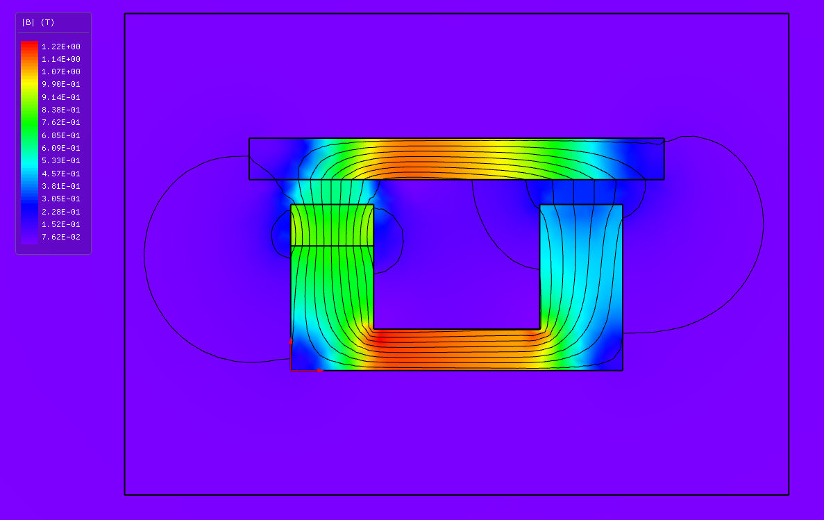
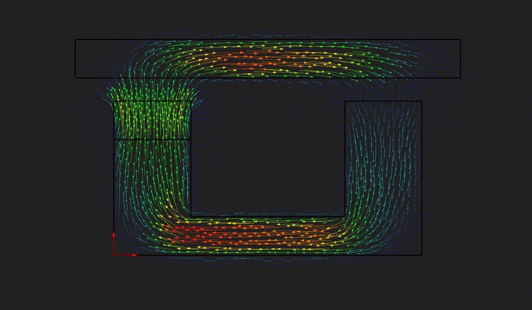
The picture is worth reading before the numbers: this loop is almost entirely self-contained. A device-width or two out, the field is already close to nothing. That fact turns out to decide the boundary study below.

Force against gap, and what the back-of-envelope misses

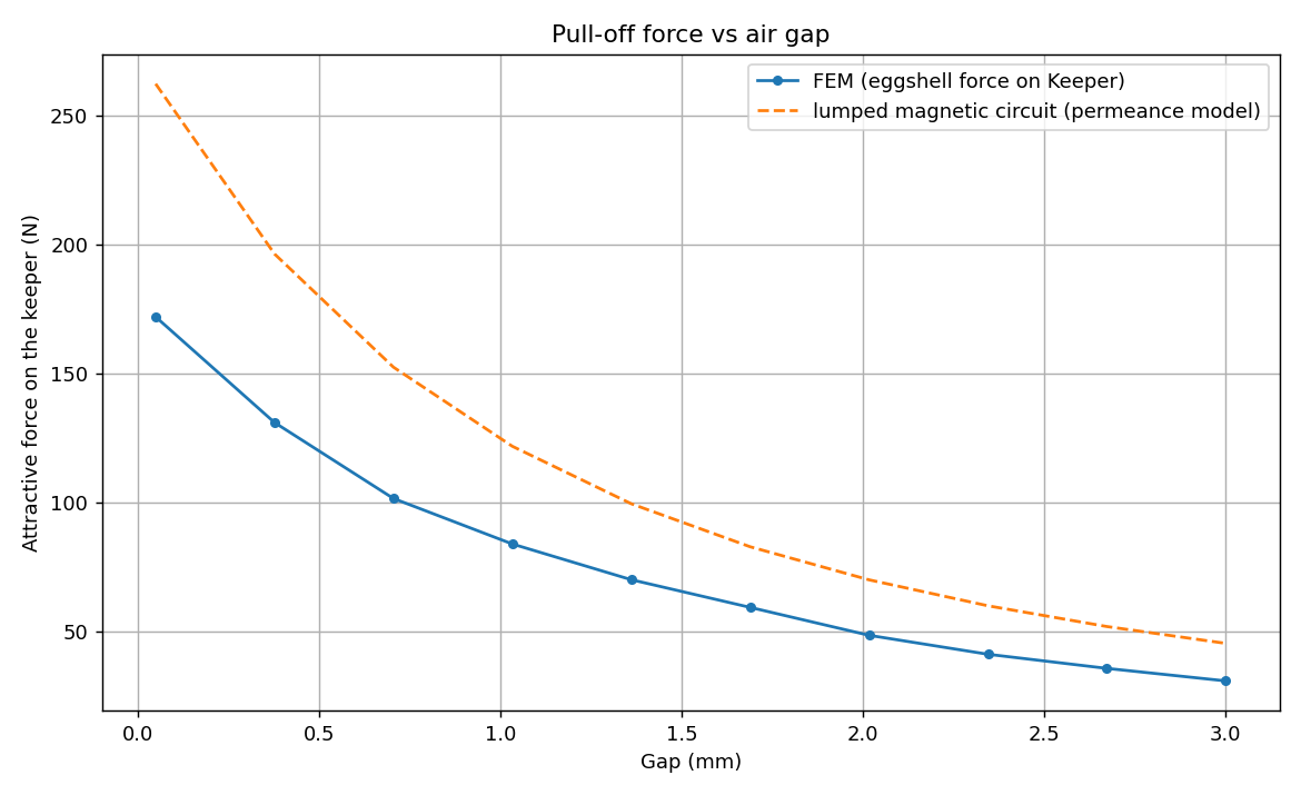
Ten static solves, from a 0.05 mm glue line to 3 mm. The force is the eggshell (Maxwell-stress) force on the Keeper region — never a contour probe, because a contour force is only valid on a path lying wholly in air and the keeper's pole faces are not.

The overlay is the classical lumped magnetic circuit. With no free current, Ampère's law around the loop is H_m·l_m + H_gap·2g = 0, the gap gives B = μ0·H_gap, and the magnet's recoil line is B = Br + μ0·μ_rec·H_m, so

B(g) = Br / (1 + mu_rec * 2g / l_m)
F(g) = B(g)^2 * A / mu0        (both gap faces)

The FEM comes in about 34 % below that at every gap, and not only at the smallest one. Two things the lumped model leaves out are real for this yoke, and both push the same way:

• Steel reluctance is not negligible. The loop's ~65 mm steel path, at a μ_r of roughly 900–1700 near this operating point, is within a factor of about 1.5 of the closed-gap air reluctance itself. That is nothing like a coil-driven electromagnet, where the gap is designed to dominate.
• The magnet's outer face is exposed straight to air, not steel-clad, so a real slice of its flux leaks there and never reaches the keeper.

The deviation does not move between the default mesh and a four-times-coarser one, so it is a modelling gap and not a mesh artefact. The example's tolerance is set to the measured number rather than to a figure a simpler model would have to hit — a yoke this short and this exposed is a fair demonstration of exactly when the classic permeance calculation stops being enough.

Three ways to close the domain

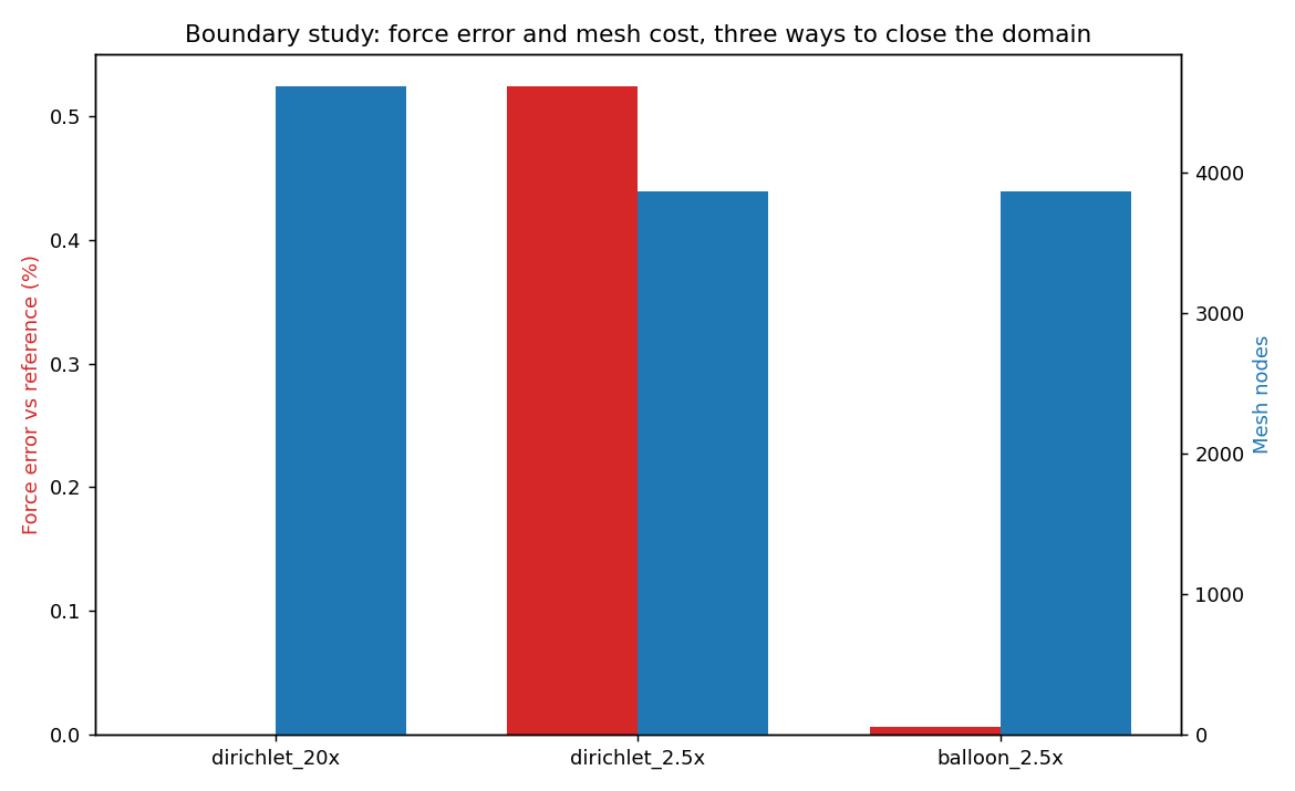
The same device at a fixed 1 mm gap, solved three ways — one process per point, because the comparison is between solved models rather than between probes on one:

Domain	Boundary	Force error vs the 20× reference	Mesh nodes
20× the device size	Dirichlet A = 0	reference	4605
2.5×	Dirichlet A = 0	0.52 %	3868 (84 %)
2.5×	far-field balloon, n = 1	0.01 %	3868 (84 %)

The honest finding is not the dramatic one. Because this yoke keeps almost all of its flux inside its own loop, even the “wrong” 2.5× Dirichlet box is already within half a percent of the 20× reference. The far-field condition still wins outright — about fifty times lower error, at identical mesh cost, because it costs nothing extra to use — but the case where it changes an answer needs a device that actually leaks into the far field: an open magnet with no return yoke, a bare coil pair, anything without this loop's own self-shielding. What this example establishes is that the balloon boundary works and is free.

As a check on the reference model's own far-field assumption, the script samples |A| along a radial line 35–380 mm above the device and fits the log-log decay slope: −1.50, against the roughly −1 a pure planar dipole would give. That gap is informational. Even a 20× Dirichlet box is itself an approximation, and this device's return yoke makes its decay a little steeper than a bare dipole's; the balloon's order n names an assumption, not a promise that a given device matches it exactly.

Demagnetisation risk

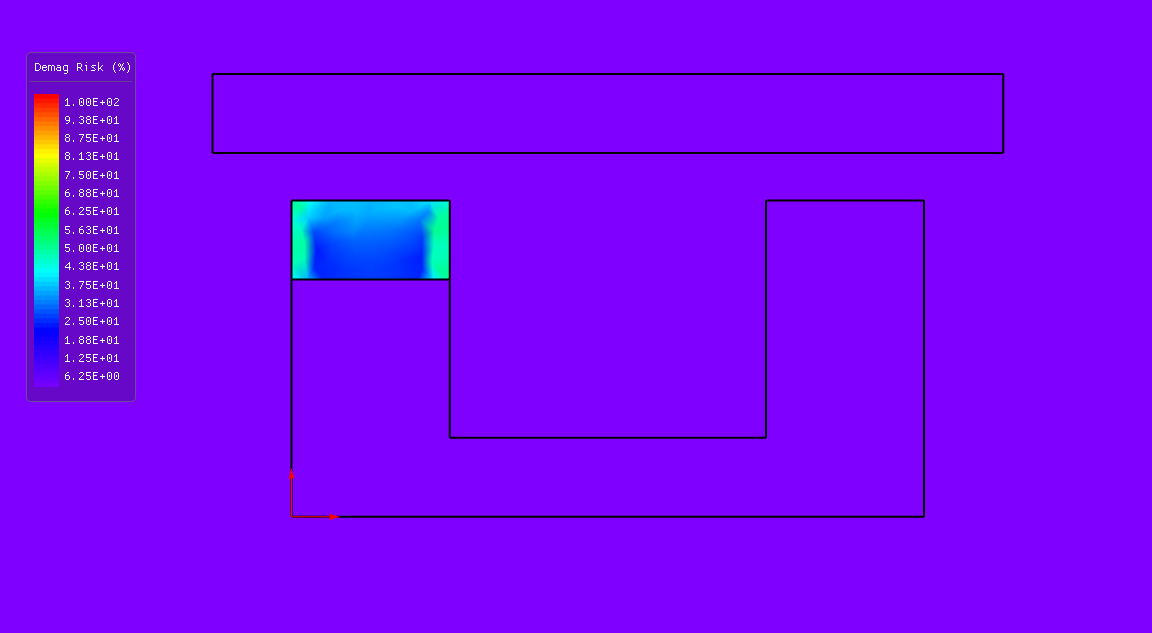
Nabla's Demag Risk field grades every point in a magnet against that material's own knee. At room temperature N42's knee sits far below this magnet's operating point at every swept gap, so the sampled risk is 0.0 % closed and open alike. What the render still shows is a small concentration — ten to twenty percent — at the magnet's two exposed top corners: the same corners identified above as the leakage path, crowding for the same reason the flux leaks there. A magnet running hotter, or graded lower, would show more, and this is the picture you would be reading if it did.

Running it

python magnet_latch.py                        # all three stages, ~35 s
python magnet_latch.py --coarse               # every mesh area x4, a fast first look
python magnet_latch.py --stage pull-off       # force vs gap only
python magnet_latch.py --stage boundary-study # the three-domain comparison only
python magnet_latch.py --stage demag          # the two field renders only

The model is small enough that JVM startup, not meshing or solving, is most of the cost — --coarse barely changes the wall time.

Try this next

• Delete the return yoke. Leave the magnet and keeper and let the flux close through air, and the boundary study stops being a formality: that is the device where the box size actually decides the answer, and where the balloon condition earns its keep.
• Warm the magnet, or grade it down. The demagnetisation render is flat at 0 % here only because N42 at room temperature has margin to spare. Bring the knee up to the operating point and the corners light up first.
• Shorten the steel path. The 34 % gap against the permeance model is mostly the yoke's own reluctance. A longer, thinner yoke widens it; a stubbier, fatter one closes it.

Two things worth copying

• Draw every shared edge once. The magnet's bottom edge is the yoke's notch top — drawn once as part of the yoke's polygon and reused, not redrawn. A duplicate coincident segment cracks the PSLG and the mesher floods one region's material over its neighbour, which solves quietly and wrongly. Nabla's rule M18 refuses the worst case (a region owning no elements at all), but a partial flood is a plausible wrong number rather than a refusal.
• The near/far air split is mesh grading, not physics. Both halves are the same μ_r = 1 air with nothing assigned to the line between them, so the field is fully continuous across it. Splitting the region only lets the far mesh coarsen with the outer box's own size, so a 20× domain does not carry sixty-four times the far-field element count for no reason.

About these numbers

This is a demonstration device, not a catalogue part. Every figure on this page came out of the run described here, at the settings the script ships with. For accuracy against a stated reference and tolerance, the validation dossier is where that question belongs.