V09 — P1 vs P2 convergence study

← Back to the validation dossier

Tier S (self-consistent) - priority P0 Reference frozen on 2026-08-14. Nabla 0.1.0, solver licence mode enforcing, run in 104.3 s.

1. Problem

Three problems whose exact solutions are already references of this dossier, each meshed at five densities and solved at both element orders, plus a fourth that exists only to close a question V01 left open. Thirty-six sub-models, and one question: does Nabla's discretization converge at the rate the theory requires, and does 2nd order earn what it costs?

Sub-model family	Physics	Exact solution first used by	Levels x orders
coax_p*_L*	planar magnetostatic, uniform Jz in a Dirichlet box	V01 (Ampère's law)	5 x 2
magnet_p*_L*	planar magnetostatic, permanent-magnet source	V13 (magnetized cylinder)	5 x 2
annulus_p*_L*	axisymmetric heat conduction, both walls held	V08 (logarithmic wall)	5 x 2
axis_p*_L*	axisymmetric magnetostatic solenoid	V01's open finding	3 x 2

The three are not interchangeable, and each is here because it can fail on its own:

• coax - a conductor of radius a = 4 mm carrying Jz = 5 MA/m^2 inside an A = 0 circle at b = 12 mm. Its B is continuous across the conductor surface, so the inscribed polygon Nabla draws for that circle costs nothing: the error a straight-sided element makes on a curved interface is proportional to the jump across it, and here there is none. The norm is taken over the whole model.
• magnet - a cylinder of radius a = 10 mm, Br = 1.2 T, mu_r = 1, magnetized along +x, inside an A = 0 circle at 3a. Its surface does carry a jump in B (a bound surface current), so the norm is taken over the exterior air ring r > 1.3a, where the same global solution is smooth. §6 says what happens if that cut is not made, and it is the practical cost of Nabla having no curved (isoparametric) element.
• annulus - the control. V08's hollow-cylinder wall, r1 = 10 mm, r2 = 40 mm, held at 100 and 20 degC. It is a rectangle in (r, z), so there is no polygon and no geometric error anywhere in it, and its solution is logarithmic, which is genuinely outside both element spaces. That second property matters more than it sounds: V08 found P2 exact on its three parabolic problems, and an exact answer has no slope to fit.

Each family's five levels scale the region area constraint and every drawn circle's segment length together, so the mesh family is geometrically similar. Measured across the five levels, h spans 3.3x and the element count 10-16x - Triangle's quality constraint gives a coarse mesh more elements than the area constraint asks for, so the achieved h is measured from the mesh rather than assumed from the request (see §6).

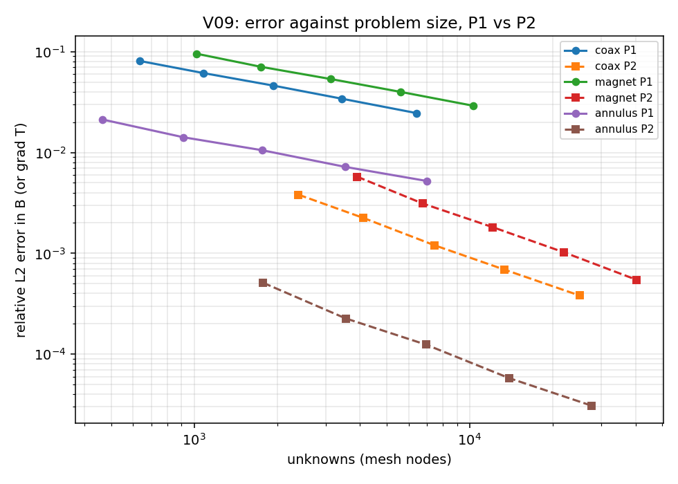
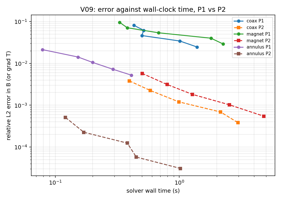
2. Reference

FEM theory, and nothing else. This is the register's tier-S case: it has no external reference by design, and it does not need one, because a convergence order is not a number a code can be tuned to. For a piecewise-smooth solution on a conforming mesh of degree-p Lagrange triangles,

|| u      - u_h      ||_L2 = O(h^(p+1))        P1 -> 2      P2 -> 3
|| grad u - grad u_h ||_L2 = O(h^p)            P1 -> 1      P2 -> 2

(Ciarlet Thm 3.2.1 for the second; Brenner & Scott Thm 4.4.20 for the extra order the first gets from duality). The tolerance is +/-0.15 on the fitted slope, which is the validation plan §3.4's own band, transcribed rather than chosen. The exact solutions are in harness/analytic.py as coax_A, magnetized_cylinder_A and annulus_T_field, each returning (u, du/dx, du/dy); for the magnetic ones B = (dA/dy, -dA/dx), so ||grad A - grad A_h|| is ||B - B_h|| and the two theory orders are being fitted on one field and its own derivative rather than on two separately post-processed quantities.

3. Nabla model and the instrument

The models are ordinary: Planar 2D / Axisymmetric 2D, SimplicialLDLT, static, linear, no motion, no circuit. solverParameters[2] carries the element order and the mesh is regenerated for every one of the thirty-six, because the order is baked into the Triangle command line.

What is not ordinary is how the error is measured, and it is the whole reason this case can say anything.

The judged quantity is a finite-element norm, not a reading. harness/fem_norms.py reads the mesh Triangle wrote (.1.node, .1.ele; six nodes per element at -o2) and the nodal degrees of freedom the solution carries, rebuilds the finite-element function with the shape functions solver/poly_2nd_order.hpp documents - including the opposite-vertex midside convention - and integrates both norms with a degree-5, 7-point quadrature on every element. Nothing is smoothed, averaged or interpolated onto anything.

Two rows exist to prove the ruler before it is used, and both are judged:

Check	Result	Why it has to pass
reconstruction_vs_probe_rel	1.73665e-16	At P1 Nabla's own getFieldInPoint("A") interpolates A linearly over the containing element, which IS the finite-element function. If the reconstruction were a different function the two could not agree to round-off.
node_coordinate_mismatch_mm	0	The mesh file's node list and the solver's own solution records have to be the same list in the same order, or every degree of freedom would be attached to the wrong node and every norm here would be meaningless while still looking like a number.

harness/fem_norms.py is also tested on its own, on structured meshes and nodal interpolants of a smooth function, with no Nabla and no JVM anywhere (validation/tests/test_fem_norms.py, 31 tests): a slope that came out right there and wrong here is the solver, and one that came out wrong there is the ruler.

Both circles are corrected before they are drawn. An inscribed regular polygon is smaller than its circle by O(1/N^2) = O(h^2) - the same order as P1's own error in B - so left alone it would flatten P2's slope to 2 while a reader watched the mesh being refined. At the magnet's coarsest level that deficit is +0.19 % of the magnet's area, and it goes straight into the dipole moment. So a circle carrying a source is drawn with the circumradius whose polygon has the circle's area (the enclosed current and the dipole moment are then exact), and a circle carrying a Dirichlet boundary with the circumradius whose polygon has the circle's logarithmic capacity (the radius the exterior solution actually sees). What is left is an N-th order multipole, which decays as (r/R)^N and is below 1e-6 at every station these norms integrate. Both corrections are derived and unit-tested against their own asymptotics.

4. Results

Quantity	Metric	Nabla	Reference	Error	Tolerance	Verdict
slope_u_coax_p1	slope	2.03369 -	2 -	0.0337	+/-0.15	PASS
slope_grad_coax_p1	slope	0.993814 -	1 -	-0.00619	+/-0.15	PASS
slope_u_coax_p2	slope	3.03682 -	3 -	0.0368	+/-0.15	PASS
slope_grad_coax_p2	slope	1.93592 -	2 -	-0.0641	+/-0.15	PASS
slope_u_magnet_p1	slope	2.03393 -	2 -	0.0339	+/-0.15	PASS
slope_grad_magnet_p1	slope	0.969675 -	1 -	-0.0303	+/-0.15	PASS
slope_u_magnet_p2	slope	2.98344 -	3 -	-0.0166	+/-0.15	PASS
slope_grad_magnet_p2	slope	1.91795 -	2 -	-0.082	+/-0.15	PASS
slope_u_annulus_p1	slope	2.01645 -	2 -	0.0164	+/-0.15	PASS
slope_grad_annulus_p1	slope	1.00755 -	1 -	0.00755	+/-0.15	PASS
slope_u_annulus_p2	slope	3.02302 -	3 -	0.023	+/-0.15	PASS
slope_grad_annulus_p2	slope	2.01289 -	2 -	0.0129	+/-0.15	PASS
reconstruction_vs_probe_rel	abs	1.73665e-16 -	0 -	1.737e-16	1e-09	PASS
node_coordinate_mismatch_mm	abs	0 mm	0 mm	0	1e-06	PASS
axis_off_axis_Bz_err_p1	report	(series)	-	-	-	REPORT
axis_off_axis_Bz_err_p2	report	(series)	-	-	-	REPORT
axis_on_axis_Bz_err_p1	report	(series)	-	-	-	REPORT
axis_on_axis_Bz_err_p2	report	(series)	-	-	-	REPORT
axis_reference_Bz_T	report	0.0202676	-	-	-	REPORT
axis_reference_Bz_offaxis_T	report	0.0202829	-	-	-	REPORT
err_grad_annulus_p1	report	(series)	-	-	-	REPORT
err_grad_annulus_p2	report	(series)	-	-	-	REPORT
err_grad_coax_p1	report	(series)	-	-	-	REPORT
err_grad_coax_p2	report	(series)	-	-	-	REPORT
err_grad_magnet_p1	report	(series)	-	-	-	REPORT
err_grad_magnet_p2	report	(series)	-	-	-	REPORT
err_u_annulus_p1	report	(series)	-	-	-	REPORT
err_u_annulus_p2	report	(series)	-	-	-	REPORT
err_u_coax_p1	report	(series)	-	-	-	REPORT
err_u_coax_p2	report	(series)	-	-	-	REPORT
err_u_magnet_p1	report	(series)	-	-	-	REPORT
err_u_magnet_p2	report	(series)	-	-	-	REPORT
nodes_annulus_p1	report	(series)	-	-	-	REPORT
nodes_annulus_p2	report	(series)	-	-	-	REPORT
nodes_coax_p1	report	(series)	-	-	-	REPORT
nodes_coax_p2	report	(series)	-	-	-	REPORT
nodes_magnet_p1	report	(series)	-	-	-	REPORT
nodes_magnet_p2	report	(series)	-	-	-	REPORT
p2_over_p1_per_dof_annulus	report	0.0236574	-	-	-	REPORT
p2_over_p1_per_dof_coax	report	0.0572534	-	-	-	REPORT
p2_over_p1_per_dof_magnet	report	0.0726495	-	-	-	REPORT
p2_over_p1_per_second_annulus	report	0.0168403	-	-	-	REPORT
p2_over_p1_per_second_coax	report	0.0383848	-	-	-	REPORT
p2_over_p1_per_second_magnet	report	0.0387911	-	-	-	REPORT
polygon_area_deficit_uncorrected_rel	report	0.00188911	-	-	-	REPORT
probe_err_grad_annulus_p1	report	(series)	-	-	-	REPORT
probe_err_grad_annulus_p2	report	(series)	-	-	-	REPORT
probe_err_grad_coax_p1	report	(series)	-	-	-	REPORT
probe_err_grad_coax_p2	report	(series)	-	-	-	REPORT
probe_err_grad_magnet_p1	report	(series)	-	-	-	REPORT
probe_err_grad_magnet_p2	report	(series)	-	-	-	REPORT
probe_err_u_annulus_p1	report	(series)	-	-	-	REPORT
probe_err_u_annulus_p2	report	(series)	-	-	-	REPORT
probe_err_u_coax_p1	report	(series)	-	-	-	REPORT
probe_err_u_coax_p2	report	(series)	-	-	-	REPORT
probe_err_u_magnet_p1	report	(series)	-	-	-	REPORT
probe_err_u_magnet_p2	report	(series)	-	-	-	REPORT
probe_slope_grad_annulus_p1	report	0.985285	-	-	-	REPORT
probe_slope_grad_annulus_p2	report	1.9255	-	-	-	REPORT
probe_slope_grad_coax_p1	report	1.43414	-	-	-	REPORT
probe_slope_grad_coax_p2	report	2.07299	-	-	-	REPORT
probe_slope_grad_magnet_p1	report	0.948602	-	-	-	REPORT
probe_slope_grad_magnet_p2	report	1.89605	-	-	-	REPORT
probe_slope_u_annulus_p1	report	2.00449	-	-	-	REPORT
probe_slope_u_annulus_p2	report	2.04019	-	-	-	REPORT
probe_slope_u_coax_p1	report	2.09032	-	-	-	REPORT
probe_slope_u_coax_p2	report	2.05735	-	-	-	REPORT
probe_slope_u_magnet_p1	report	1.99476	-	-	-	REPORT
probe_slope_u_magnet_p2	report	1.90964	-	-	-	REPORT
slope_grad_annulus_p1_finest3	report	1.00704	-	-	-	REPORT
slope_grad_annulus_p2_finest3	report	2.00046	-	-	-	REPORT
slope_grad_coax_p1_finest3	report	1.02267	-	-	-	REPORT
slope_grad_coax_p2_finest3	report	1.8673	-	-	-	REPORT
slope_grad_magnet_p1_finest3	report	0.97559	-	-	-	REPORT
slope_grad_magnet_p2_finest3	report	1.92282	-	-	-	REPORT
slope_u_annulus_p1_finest3	report	2.01098	-	-	-	REPORT
slope_u_annulus_p2_finest3	report	2.99627	-	-	-	REPORT
slope_u_coax_p1_finest3	report	2.07736	-	-	-	REPORT
slope_u_coax_p2_finest3	report	2.83745	-	-	-	REPORT
slope_u_magnet_p1_finest3	report	2.06431	-	-	-	REPORT
slope_u_magnet_p2_finest3	report	3.00025	-	-	-	REPORT
wall_s_annulus_p1	report	(series)	-	-	-	REPORT
wall_s_annulus_p2	report	(series)	-	-	-	REPORT
wall_s_coax_p1	report	(series)	-	-	-	REPORT
wall_s_coax_p2	report	(series)	-	-	-	REPORT
wall_s_magnet_p1	report	(series)	-	-	-	REPORT
wall_s_magnet_p2	report	(series)	-	-	-	REPORT

• axis_off_axis_Bz_err_p1: extracted but not frozen in expected.json - reported only
• axis_off_axis_Bz_err_p2: extracted but not frozen in expected.json - reported only
• axis_on_axis_Bz_err_p1: extracted but not frozen in expected.json - reported only
• axis_on_axis_Bz_err_p2: extracted but not frozen in expected.json - reported only
• axis_reference_Bz_T: extracted but not frozen in expected.json - reported only
• axis_reference_Bz_offaxis_T: extracted but not frozen in expected.json - reported only
• err_grad_annulus_p1: extracted but not frozen in expected.json - reported only
• err_grad_annulus_p2: extracted but not frozen in expected.json - reported only
• err_grad_coax_p1: extracted but not frozen in expected.json - reported only
• err_grad_coax_p2: extracted but not frozen in expected.json - reported only
• err_grad_magnet_p1: extracted but not frozen in expected.json - reported only
• err_grad_magnet_p2: extracted but not frozen in expected.json - reported only
• err_u_annulus_p1: extracted but not frozen in expected.json - reported only
• err_u_annulus_p2: extracted but not frozen in expected.json - reported only
• err_u_coax_p1: extracted but not frozen in expected.json - reported only
• err_u_coax_p2: extracted but not frozen in expected.json - reported only
• err_u_magnet_p1: extracted but not frozen in expected.json - reported only
• err_u_magnet_p2: extracted but not frozen in expected.json - reported only
• nodes_annulus_p1: extracted but not frozen in expected.json - reported only
• nodes_annulus_p2: extracted but not frozen in expected.json - reported only
• nodes_coax_p1: extracted but not frozen in expected.json - reported only
• nodes_coax_p2: extracted but not frozen in expected.json - reported only
• nodes_magnet_p1: extracted but not frozen in expected.json - reported only
• nodes_magnet_p2: extracted but not frozen in expected.json - reported only
• p2_over_p1_per_dof_annulus: extracted but not frozen in expected.json - reported only
• p2_over_p1_per_dof_coax: extracted but not frozen in expected.json - reported only
• p2_over_p1_per_dof_magnet: extracted but not frozen in expected.json - reported only
• p2_over_p1_per_second_annulus: extracted but not frozen in expected.json - reported only
• p2_over_p1_per_second_coax: extracted but not frozen in expected.json - reported only
• p2_over_p1_per_second_magnet: extracted but not frozen in expected.json - reported only
• polygon_area_deficit_uncorrected_rel: extracted but not frozen in expected.json - reported only
• probe_err_grad_annulus_p1: extracted but not frozen in expected.json - reported only
• probe_err_grad_annulus_p2: extracted but not frozen in expected.json - reported only
• probe_err_grad_coax_p1: extracted but not frozen in expected.json - reported only
• probe_err_grad_coax_p2: extracted but not frozen in expected.json - reported only
• probe_err_grad_magnet_p1: extracted but not frozen in expected.json - reported only
• probe_err_grad_magnet_p2: extracted but not frozen in expected.json - reported only
• probe_err_u_annulus_p1: extracted but not frozen in expected.json - reported only
• probe_err_u_annulus_p2: extracted but not frozen in expected.json - reported only
• probe_err_u_coax_p1: extracted but not frozen in expected.json - reported only
• probe_err_u_coax_p2: extracted but not frozen in expected.json - reported only
• probe_err_u_magnet_p1: extracted but not frozen in expected.json - reported only
• probe_err_u_magnet_p2: extracted but not frozen in expected.json - reported only
• probe_slope_grad_annulus_p1: extracted but not frozen in expected.json - reported only
• probe_slope_grad_annulus_p2: extracted but not frozen in expected.json - reported only
• probe_slope_grad_coax_p1: extracted but not frozen in expected.json - reported only
• probe_slope_grad_coax_p2: extracted but not frozen in expected.json - reported only
• probe_slope_grad_magnet_p1: extracted but not frozen in expected.json - reported only
• probe_slope_grad_magnet_p2: extracted but not frozen in expected.json - reported only
• probe_slope_u_annulus_p1: extracted but not frozen in expected.json - reported only
• probe_slope_u_annulus_p2: extracted but not frozen in expected.json - reported only
• probe_slope_u_coax_p1: extracted but not frozen in expected.json - reported only
• probe_slope_u_coax_p2: extracted but not frozen in expected.json - reported only
• probe_slope_u_magnet_p1: extracted but not frozen in expected.json - reported only
• probe_slope_u_magnet_p2: extracted but not frozen in expected.json - reported only
• slope_grad_annulus_p1_finest3: extracted but not frozen in expected.json - reported only
• slope_grad_annulus_p2_finest3: extracted but not frozen in expected.json - reported only
• slope_grad_coax_p1_finest3: extracted but not frozen in expected.json - reported only
• slope_grad_coax_p2_finest3: extracted but not frozen in expected.json - reported only
• slope_grad_magnet_p1_finest3: extracted but not frozen in expected.json - reported only
• slope_grad_magnet_p2_finest3: extracted but not frozen in expected.json - reported only
• slope_u_annulus_p1_finest3: extracted but not frozen in expected.json - reported only
• slope_u_annulus_p2_finest3: extracted but not frozen in expected.json - reported only
• slope_u_coax_p1_finest3: extracted but not frozen in expected.json - reported only
• slope_u_coax_p2_finest3: extracted but not frozen in expected.json - reported only
• slope_u_magnet_p1_finest3: extracted but not frozen in expected.json - reported only
• slope_u_magnet_p2_finest3: extracted but not frozen in expected.json - reported only
• wall_s_annulus_p1: extracted but not frozen in expected.json - reported only
• wall_s_annulus_p2: extracted but not frozen in expected.json - reported only
• wall_s_coax_p1: extracted but not frozen in expected.json - reported only
• wall_s_coax_p2: extracted but not frozen in expected.json - reported only
• wall_s_magnet_p1: extracted but not frozen in expected.json - reported only
• wall_s_magnet_p2: extracted but not frozen in expected.json - reported only

All twelve slopes land on theory, and the worst of them is 0.082 off an integer against a +/-0.15 band. Read as a block:

Problem	P1 u (2)	P1 grad (1)	P2 u (3)	P2 grad (2)
coax	2.03369	0.993814	3.03682	1.93592
magnet	2.03393	0.969675	2.98344	1.91795
annulus	2.01645	1.00755	3.02302	2.01289

Three problems, three different physics, two element orders, four theoretical orders - twelve independent fits, no free parameter anywhere, and the largest deviation is 4 % of the quantity being fitted.

Does P2 pay for itself?

That is the question the plan actually asks, and "is it more accurate on the same mesh" is not it - P2 is more accurate on the same mesh and it is also more expensive on it. The honest comparison is at equal cost, so each order's own error curve is interpolated in log-log to the other's finest budget:

Problem	error ratio P2/P1 at equal unknowns	at equal wall time
coax	0.0572534	0.0383848
magnet	0.0726495	0.0387911
annulus	0.0236574	0.0168403

So on these three smooth problems P2 is 14 to 42 times more accurate per unknown, and 26 to 59 times more accurate per second of solver time. It is worth being precise about what that does and does not license: all three solutions here are smooth, all three geometries are convex or annular, and none of them has a re-entrant corner, a sliding band or a saturating material. The plan predicted "for smooth problems yes, per unknown and per second; near re-entrant corners the advantage shrinks", and this case measures the first half and does not test the second. §7 says so again.

5. Discussion - the ruler is not the result

The validation plan V09 was written after V05 spent a chapter measuring a Maxwell-stress line integral rather than the field it was applied to, and it carries the lesson forward as an instruction: fit slopes on a proven estimator, and publish the estimator's own convergence beside the solution's.

The estimator a user actually has is getFieldInPoint. Two predictions about it were written down before this case was run, from reading the code rather than from any measurement:

1. Results.calcAaux interpolates A linearly over the triangle the probe search returns. At 1st order that triangle is the element and the interpolation is the finite-element function - so the probe is exact. At 2nd order the search runs over P2Render.displayElements(), the four-way split of each quadratic element, so the probe returns a piecewise-linear interpolant of a quadratic solution on sub-triangles of size h/2. That costs O(h^2), which is below the O(h^3) being measured. The probe should report slope 2 for a perfect P2 solver.
2. calcBxAux interpolates the nodally averaged Bx/By, which is a recovery operator, and a recovery operator is superconvergent at interior nodes at P1. The probe should report a slope above 1, and an error below the true one, at P1.

Both hold, and the numbers are worth quoting:

	probe slope, u	probe slope, grad	probe error / true error, finest level
coax P1	2.09032	1.43414	A 1.01x, B 0.25x
coax P2	2.05735	2.07299	A 55x, B 0.66x
magnet P1	1.99476	0.948602	A 0.99x, B 0.22x
magnet P2	1.90964	1.89605	A 19x, B 0.88x
annulus P1	2.00449	0.985285	T 1.10x, grad T 0.38x
annulus P2	2.04019	1.9255	T 104x, grad T 1.32x

Three things follow, and they are the practical output of this chapter.

At 1st order the point probe is the solution. Its A/T error reproduces the finite-element norm to 1 % (1.01x, 0.99x, 1.10x) and its slope is 1.99-2.09. Nothing is lost by reading a P1 solution through it.

At 2nd order the A/T probe has a floor of its own, and it is large. On the finest annulus mesh the true error is 7.1e-8 and the probe reads 7.4e-6 - 104 times bigger - and its fitted slope is 2.04019 where the solution's is 3.02302. A user who refines a P2 model and watches the probe will conclude their solver is 2nd order in A when it is 3rd, and will stop refining a decade too early. This is a display-mesh limitation, not a solver one - the degrees of freedom are right, and every integral post-processing path already reads them properly - but it is the number to know before quoting a P2 point probe.

The B probe is better than the field it comes from, at P1. It reads 0.22x to 0.38x the true element-wise error, because nodal averaging is a recovery operator; its fitted slope runs 0.95 to 1.43 rather than a clean 1. That is good news for a user and bad news for anyone fitting a convergence order through it: it is a different approximation, not a measurement of the one being studied. It is also the reason this case does not judge a single row on a probe.

6. What had to be got right, and what it cost

h is measured, not requested. The five levels ask for element sizes in the ratio 1 : 1/sqrt2 : 1/2 : ..., but Triangle's quality constraint gives a coarse mesh more elements than the area constraint alone would, so the achieved sizes span 3.3x where the request spans 4x. Every slope here is fitted against h = sqrt(4 A / (sqrt3 E)) computed from the mesh that was actually generated. Fitting against the requested h instead would have moved every slope by about 15 % and turned four passing rows into failures - a case that measured its own request rather than its own mesh.

The magnet's norm is taken outside the magnet, and that is not a convenience. Nabla has no isoparametric element: a P2 triangle is straight-sided, and the magnet surface reaches it as a polygon. Where B jumps across that surface, the sliver between polygon and circle is wrong by O(1) over a width O(h^2), which contributes O(h) to a relative L2 error in B at every element order. Fitted through the magnet surface, P2's grad slope would be measuring the polygon. The cut is placed on a region boundary at 1.3a, so it runs between elements and never through one. This is a real limitation and it belongs in §5 of the manual: on a curved material interface, Nabla's practical order in B is set by how finely the interface is polygonised, not by the element order - which is one more reason the airgap of a machine model wants segments, not just area constraints.

Both problems with circles need their circumradius corrected. See §3. Had they not been, the coarsest magnet model would have carried +0.19 % too little magnet, falling as h^2 - indistinguishable from a discretization error, and exactly the size that caps a 3rd-order method at 2nd.

The probe takes single-precision coordinates. getFieldInPointAPI declares float x, float y, so a station is answered at the float32 rounding of the point it was given - a 6e-8 relative shift, which on a field gradient is the whole difference between two readings that should be identical. The reconstruction check rounds its stations to float32 before asking either instrument, so what it reports is the reconstruction and not the coordinate conversion. Worth knowing before comparing two probe readings that ought to agree exactly.

7. V01's open question, answered

V01 published, without a verdict, that B_z probed exactly on the symmetry axis of an axisymmetric model reads +40 % at P1 against -0.08 % at P2, that refining does not help, and that V09 should measure it as a convergence study. Here it is: an axisymmetric solenoid (r = 20..24 mm, +/-30 mm long, NI = 1200 A), three mesh levels, both orders, read twice per solve - once at r = 0 and once at r = 2 mm. The reference is the exact on-axis field of a rectangular-section coil, 0.0202676 T, and the exact off-axis value from the same current distribution.

Level (coarse -> fine)	P1 on the axis	P1 at r = 2 mm	P2 on the axis	P2 at r = 2 mm
1	+5.63 %	+3.66 %	-0.81 %	-0.85 %
2	-2.56 %	-1.22 %	-0.83 %	-0.82 %
3	+28.98 %	-1.70 %	-0.82 %	-0.83 %

The P1 on-axis reading does not converge - it gets worse. The same solve read two millimetres off the axis converges normally, and P2 is flat to 0.02 % across the sweep at both stations. The common -0.8 % in the P2 column is the Dirichlet box this model is truncated with, which is the same for every row and cancels out of the comparison entirely: what is left in the P1 column is the recovery.

The mechanism is the one V01 named. An axisymmetric magnetic solution stores u = r*A_phi, and B_z = (1/r) du/dr at r = 0 is a 0/0 that only P2's axis-node Hessian recovery resolves; at P1 the answer depends on which element the probe happened to land in and how close its nodes are to the axis, which is why a finer mesh can be worse. Guidance: never read B_z on the axis of a P1 axisymmetric model. Read it a millimetre or two off, or use P2. Integral quantities are unaffected at either order (V01 measured that separately).

8. Limitations

• Three smooth problems on three well-behaved geometries. No re-entrant corner, no saturating material, no sliding band, no transient. The "P2 pays for itself" numbers in §4 are for smooth problems and the chapter says so; the plan's own expectation is that the advantage shrinks near a re-entrant corner, and this case does not test that.
• Element order is not the only P2 cost, and the others are not measured here. The second-order element specification fixes what P2 gives up: the averaging sliding band only - the legacy stitch band is rejected outright - axisymmetric + skew rejected at both orders, and rotor-bar/stator skew at P2 costing about 6.6x the nnz and 11x the wall time per step against the same skewed P1 run. A P2 machine model also needs its sliding-band ring subdivided more finely than the shipped arcLength / (0.5 * airGap) default, which is a P1 default: V05 measured the element layer touching the band ring carrying 38x and 81x the numerical noise of a layer one region away until the ring was refined 4x. None of that is exercised here, and a reader weighing P2 should read the accuracy claim above together with that list.
• The norms are L2 norms over a domain. They say nothing about a local quantity at a corner, a force on a contour, or a torque - each of which has its own estimator, and V02, V05 and V15 are the chapters about those.
• Only the magnetic and thermal static kernels. Time-harmonic P2 and transient P2 exist (time_harmonic_p2, the thermal transient) and are not measured here; V19 is the time-integration order study.

9. Reproduce

cd validation
python -m harness.run_case V09
python -m pytest tests/test_fem_norms.py     # the ruler, without Nabla

The eighteen 1st-order sub-models are reproducible on the free tier; the 2nd-order ones need Feature.CORE_PRO. All thirty-six run in 104.3 s.

Every series quoted in the tables above - the five-level error curves, the probe curves, the node counts, the wall times and the axis sweep - is written out in full to artifacts/series/*.json, and the per-sub-model mesh statistics are in artifacts/results.json under provenance.sub_models.

Sub-model	Element order	Nodes	Elements
coax_p1_L0	P1	634	1125
coax_p1_L1	P1	1077	1952
coax_p1_L2	P1	1935	3585
coax_p1_L3	P1	3441	6480
coax_p1_L4	P1	6407	12247
coax_p2_L0	P2	2392	1125
coax_p2_L1	P2	4105	1952
coax_p2_L2	P2	7454	3585
coax_p2_L3	P2	13361	6480
coax_p2_L4	P2	25060	12247
magnet_p1_L0	P1	1021	1863
magnet_p1_L1	P1	1749	3246
magnet_p1_L2	P1	3125	5895
magnet_p1_L3	P1	5622	10742
magnet_p1_L4	P1	10282	19855
magnet_p2_L0	P2	3904	1863
magnet_p2_L1	P2	6743	3246
magnet_p2_L2	P2	12144	5895
magnet_p2_L3	P2	21985	10742
magnet_p2_L4	P2	40418	19855
annulus_p1_L0	P1	463	856
annulus_p1_L1	P1	914	1723
annulus_p1_L2	P1	1770	3400
annulus_p1_L3	P1	3540	6877
annulus_p1_L4	P1	6982	13675
annulus_p2_L0	P2	1781	856
annulus_p2_L1	P2	3550	1723
annulus_p2_L2	P2	6939	3400
annulus_p2_L3	P2	13956	6877
annulus_p2_L4	P2	27638	13675
axis_p1_L0	P1	1682	3226
axis_p1_L1	P1	3220	6269
axis_p1_L2	P1	6304	12341
axis_p2_L0	P2	6589	3226
axis_p2_L1	P2	12708	6269
axis_p2_L2	P2	24948	12341

Date	Change	Reason
2026-08-14	frozen at creation	Every reference here is an integer from FEM theory and every tolerance is the plan's own +/-0.15 slope band. Both were written down before the case was run, and neither depends on anything Nabla returned.