V12 — Skin effect: round conductor, slab and slot conductor

← Back to the validation dossier

Tier A (analytic) — priority P0 Reference frozen on 2026-08-11. Nabla 0.1.0, solver licence mode enforcing, run in 52.1 s.

1. Problem

Three conductors, one equation, five decades of frequency.

Eddy currents in a linear conductor obey laplacian(J) = j omega mu sigma J, and the only length in it is the skin depth delta = sqrt(2/(omega mu sigma)). Three geometries reduce it to one dimension, and all three then have closed-form solutions that have been in the literature for a century:

Family	Model	Swept	delta runs from
Round wire	copper, a = 1.5 mm, isolated in a 10 a air disc	2, 20, 200, 2000, 20000 Hz	31 a down to a/3.2
Slab	copper, 2d = 10 mm thick, in a 200 kA/m RMS tangential field	50, 500, 5000 Hz	1.9 d down to 0.19 d
Slot bar	copper, 20 x 5 mm, filling an open slot in infinitely permeable iron	5, 50, 200, 500 Hz	1.5 h down to 0.15 h

plus a resolution sweep: the 20 kHz wire meshed at 1, 2, 4, 8 and 16 elements per skin depth. Sixteen sub-models in all, every one planar 2D, linear, P1, time-harmonic with eddy currents on.

The three models are one-dimensional problems built in a two-dimensional code, and what makes them so is which boundaries carry no condition at all.

• Infinitely permeable iron is the natural boundary. A boundary with no BC satisfies dA/dn = 0, i.e. H_t = 0, i.e. flux entering perpendicular — which is exactly what an infinitely permeable wall does. The slot's two side walls and its bottom therefore carry nothing, and that is the model rather than an omission. Only the slot mouth is Dirichlet.
• A prescribed tangential field is Ampère's law plus one natural boundary. The slab's top boundary is natural (H_x = 0 on it) and a stranded coil of total current I sits between it and the slab, so the field at the slab surface is I/L exactly — no inhomogeneous Neumann condition anywhere, and no dependence on what the slab itself induces, because the drive coil is not conducting.
• A slab's symmetry plane is A = 0, not a natural boundary: J is odd about it and J = -j omega sigma A in a source-free conductor. Modelling it the other way solves a slab with an insulating mid-plane, which is a different problem with a different answer.

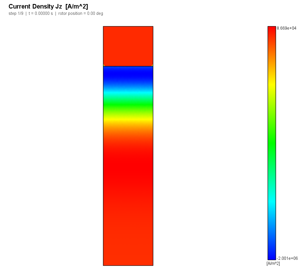
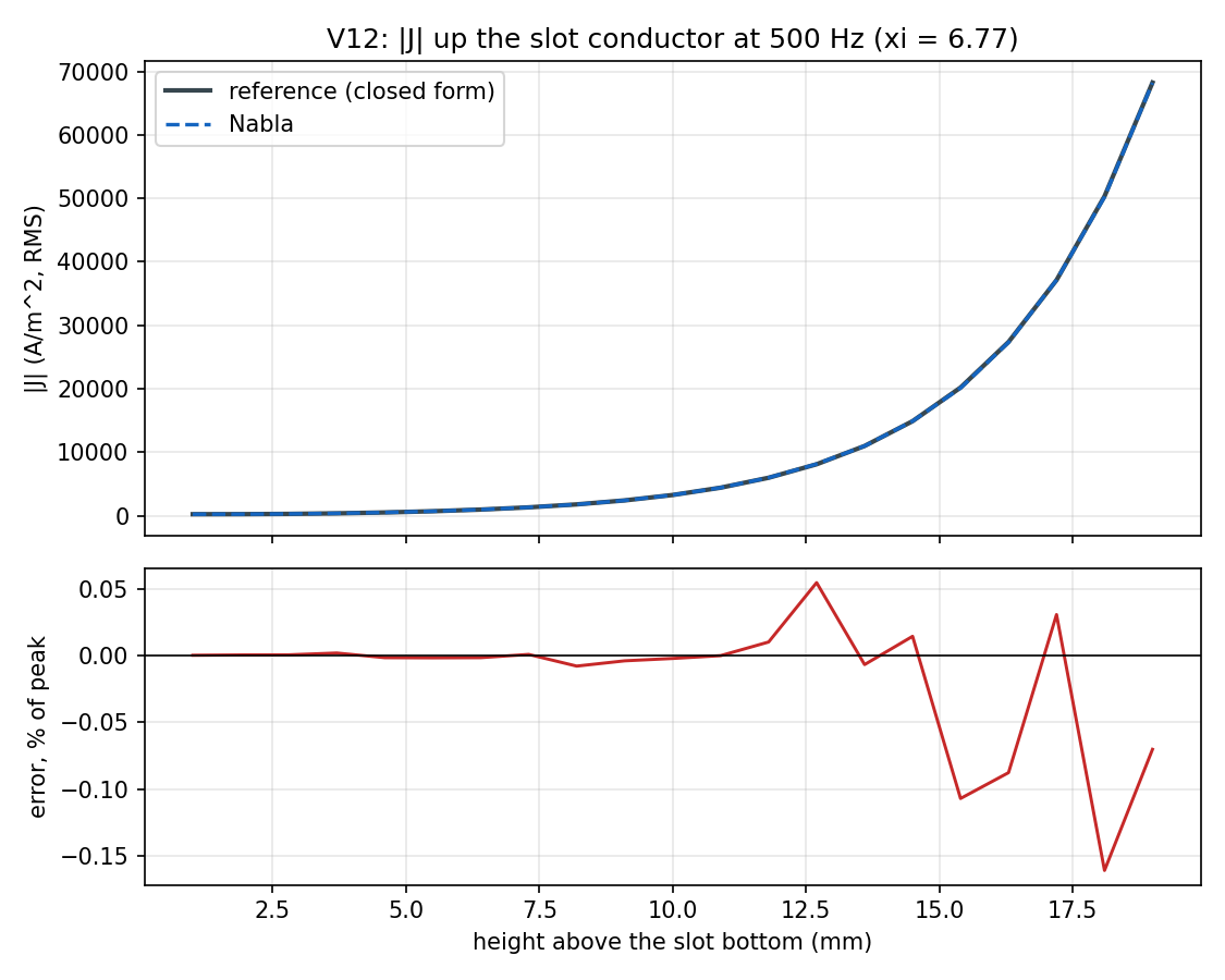
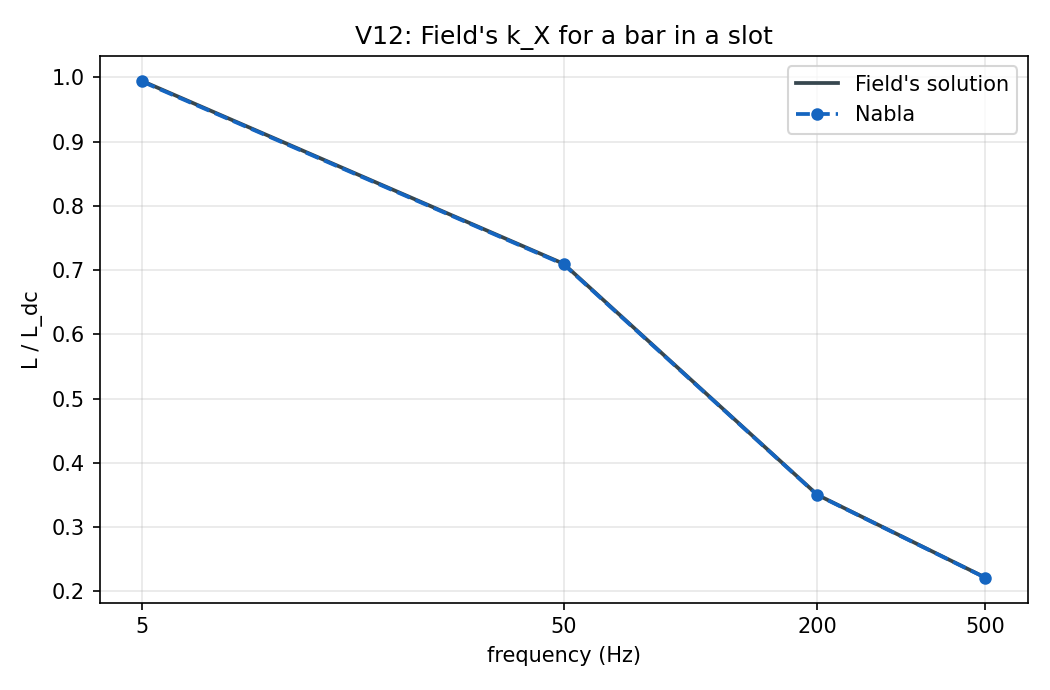
The bar is the whole picture — the slot mouth is the strip above it. At xi = h/delta = 6.77 the current density at the top of the bar is three hundred times what it is at the bottom, and its sign is opposite: the deep part of the bar is carrying return current at this instant. That is what raises the bar's resistance 6.8-fold and drops its slot leakage to 0.22 of the DC value.

2. Reference

Closed form throughout, derived in the case's reference notes and evaluated by harness/analytic.py at run time; a disagreement with the frozen numbers is reported as DRIFT and fails the case.

round wire   Z_int = (k/(2 pi a sigma)) J0(ka)/J1(ka),   k = (1-j)/delta
             R_ac/R_dc = (xi/2)(ber bei' - bei ber')/(ber'^2 + bei'^2)
             L_int/L_dc = (4/xi)(ber ber' + bei bei')/(ber'^2 + bei'^2)
             R_dc = 1/(sigma pi a^2),  L_dc = mu0/(8 pi),  xi = sqrt(2) a/delta

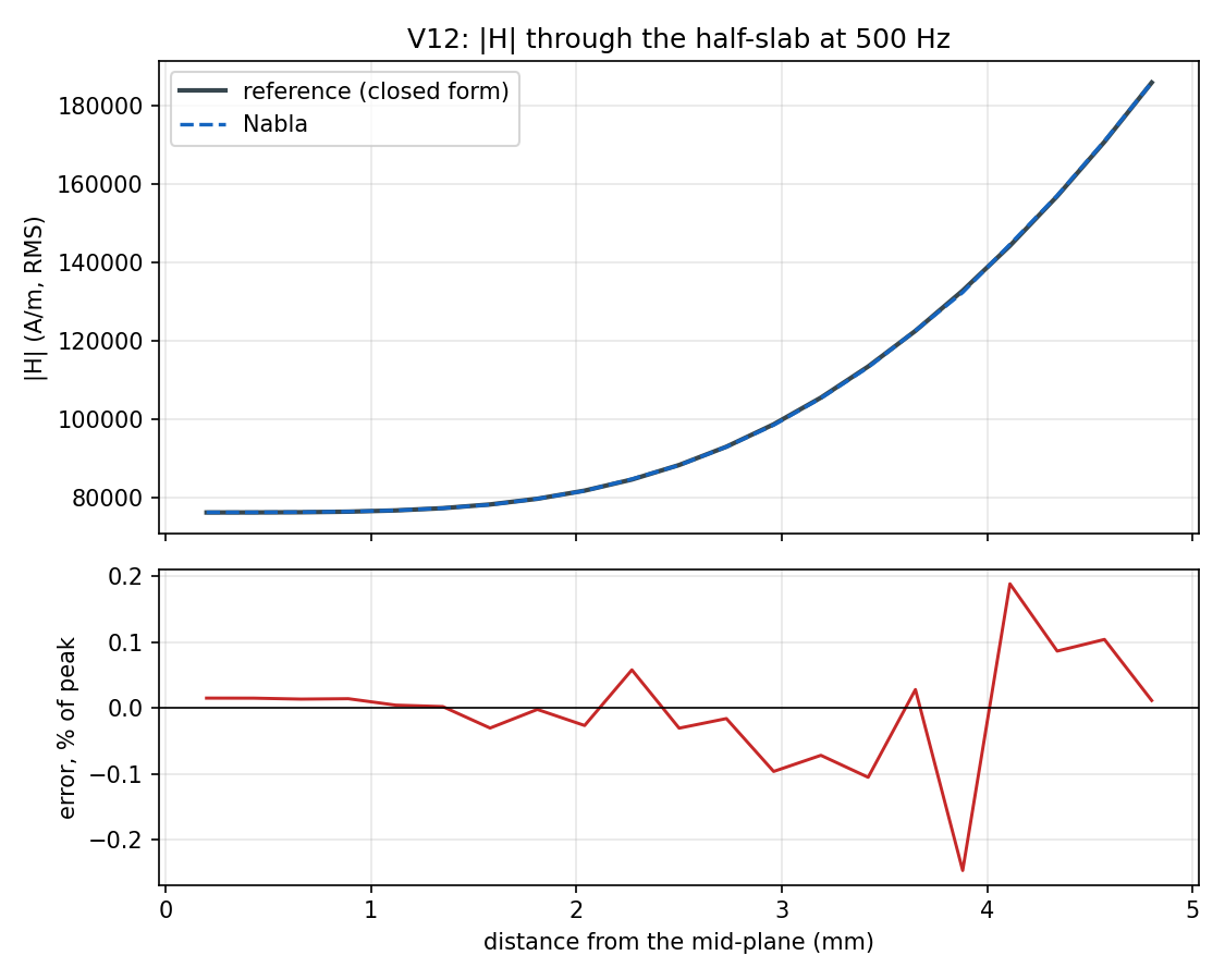
slab         H(x) = H_s cosh(gamma x)/cosh(gamma d),     gamma = (1+j)/delta
             P = (2 H_rms^2/(sigma delta))(sinh 2xi - sin 2xi)/(cosh 2xi + cos 2xi)

slot bar     J(y) proportional to cosh(gamma y)
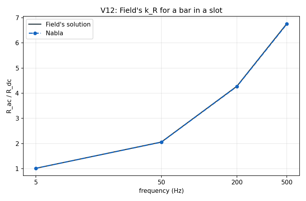
             k_R = xi (sinh 2xi + sin 2xi)/(cosh 2xi - cos 2xi)
             k_X = (3/2xi)(sinh 2xi - sin 2xi)/(cosh 2xi - cos 2xi)
             R_dc = 1/(sigma b h),  L_dc = mu0 h/(3 b),  xi = h/delta

Resistance and inductance are the complex Poynting theorem and nothing else: R = P/I_rms^2 and L = 2<W_m>/I_rms^2, with <W_m> the time-average energy stored inside the conductor. Both are region integrals, so this case reads them straight off Joule Losses and Field Energy and does no post-processing of its own.

The round conductor's reference is derived twice. The Kelvin-function form and the complex-Bessel form are different books' algebra for the same physics, and the case judges them against each other before it asks the solver anything: analytic_selfcheck_max_rel_err = 2.25375e-13.

Source statement as frozen: Closed form throughout, for three geometries whose eddy-current problem is one-dimensional. (1) ROUND WIRE, isolated, radius a = 1.5 mm, copper sigma = 5.8e7 S/m, mu_r = 1: the internal impedance is Z = (k/(2 pi a sigma)) J0(ka)/J1(ka) with k = (1-j)/delta, equivalently R_ac/R_dc = (xi/2)(ber bei' - bei ber')/(ber'^2 + bei'^2) and L_int/L_dc = (4/xi)(ber ber' + bei bei')/(ber'^2 + bei'^2) at xi = sqrt(2) a/delta, against R_dc = 1/(sigma pi a^2) = 2.43916e-3 ohm/m and L_dc = mu0/(8 pi) = 50 nH/m; the current density is J(r) = I k J0(kr)/(2 pi a J1(ka)). (2) SLAB of half-thickness d = 5 mm in a tangential field H_s on both faces: H(x) = H_s cosh(gamma x)/cosh(gamma d) with gamma = (1+j)/delta, and a loss of (2 H_rms^2/(sigma delta))(sinh 2xi - sin 2xi)/(cosh 2xi + cos 2xi) per unit face area at xi = d/delta, of which the modelled half-slab dissipates half. (3) BAR filling an open slot, h = 20 mm by b = 5 mm (Field's solution): k_R = xi(sinh 2xi + sin 2xi)/(cosh 2xi - cos 2xi) and k_X = (3/2xi)(sinh 2xi - sin 2xi)/(cosh 2xi - cos 2xi) at xi = h/delta, against R_dc = 1/(sigma b h) = 1.72414e-4 ohm/m and L_dc = mu0 h/(3 b) = 1.67552 uH/m, with J(y) proportional to cosh(gamma y). Impedances are defined by the complex Poynting theorem and nothing else: R = P/I_rms^2 and L = 2/I_rms^2, both read straight off a region integral. All of it is derived and evaluated in harness/analytic.py (section: skin effect); tolerances are transcribed from the validation plan, case V12. The two source-current rows are the closed form of the problem Nabla's impressed-current-density drive ACTUALLY solves - a voltage source of I_source * R_dc per metre - and are derived in the case's reference notes.

3. Nabla model

Built entirely through nabla_api by build.py in this directory — no GUI step, no manual edit. Each sub-model is meshed at sixteen elements per its own skin depth, floored by a geometric rule so that a 2 Hz model whose skin depth is thirty times the wire still resolves the wire. Why sixteen and not the four the plan asks for is §5, and it was decided before the run: the reasoning is written out in build.py above ELEMENTS_PER_SKIN_DEPTH.

Sub-model	Element order	Nodes	Elements
round_2Hz	P1	1803	3541
round_20Hz	P1	1803	3541
round_200Hz	P1	1803	3541
round_2kHz	P1	3144	6223
round_20kHz	P1	18831	37597
round_res1	P1	1382	2699
round_res2	P1	1612	3159
round_res4	P1	2438	4811
round_res8	P1	5712	11359
slab_50Hz	P1	97	147
slab_500Hz	P1	338	596
slab_5kHz	P1	2816	5420
slot_5Hz	P1	340	611
slot_50Hz	P1	615	1136
slot_200Hz	P1	2290	4409
slot_500Hz	P1	5595	10926

The four round_res* models opt out of the geometric floor — a sub-model whose job is to be under-resolved has to be allowed to be — and out of the 60-chord minimum on the conductor circle with it, because ringing a coarse conductor with fine boundary elements would let that sweep flatter itself.

Time-harmonic is a Core Pro feature, so this case does not run on the free tier: solverSettings("Time-Harmonic", ...) refuses without it. Every model is P1 and comfortably inside the free tier's node cap; it is the physics that is gated, not the size. The models are published beside this chapter under artifacts/models/.

4. Results

Quantity	Metric	Nabla	Reference	Error	Tolerance	Verdict
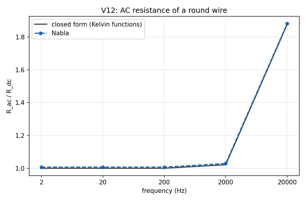
round_R_ratio_vs_f	profile	min=1.007, max=1.882, rms=1.237 -	min=1, max=1.877, rms=1.23 -	L2 +0.560 %, max +0.401 %	L2 2.000 %, max 2.000 %	PASS
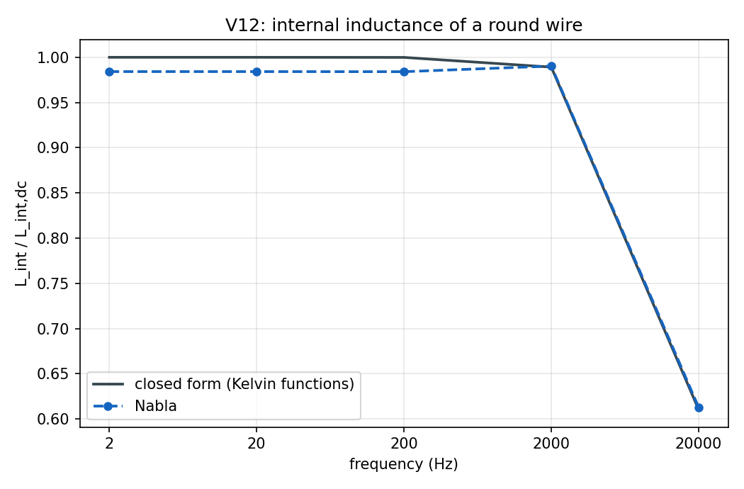
round_L_ratio_vs_f	profile	min=0.613, max=0.9903, rms=0.9233 -	min=0.6105, max=1, rms=0.9328 -	L2 +1.320 %, max +1.582 %	L2 2.000 %, max 3.000 %	PASS
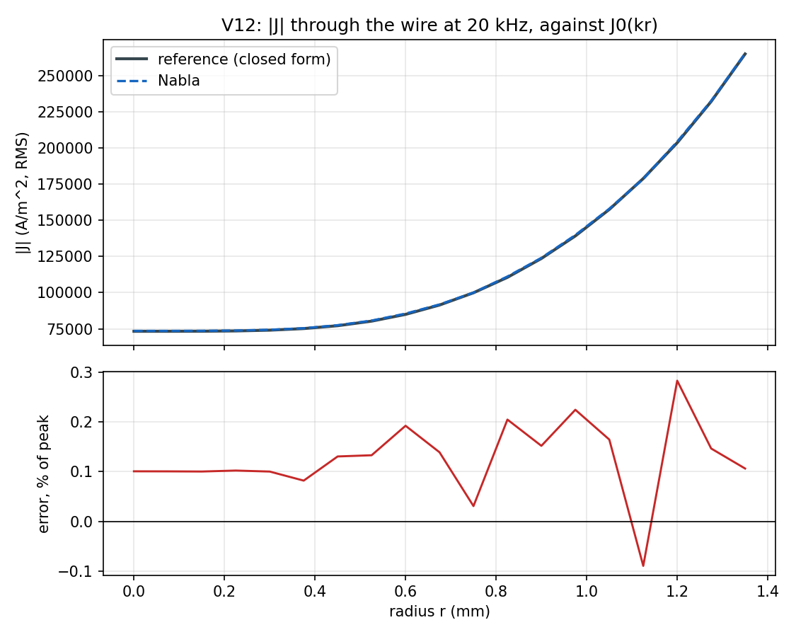
round_J_profile_per_amp	profile	min=7.354e+04, max=2.652e+05, rms=1.34e+05 1/m^2	min=7.328e+04, max=2.65e+05, rms=1.337e+05 1/m^2	L2 +0.292 %, max +0.283 %	L2 3.000 %, max 5.000 %	PASS
round_source_current_ratio_vs_f	profile	min=0.03938, max=0.9973, rms=0.7806 -	min=0.03942, max=1, rms=0.7825 -	L2 +0.253 %, max +0.268 %	L2 3.000 %, max 3.000 %	PASS
round_resolution_R_ratio	profile	min=1.264, max=1.882, rms=1.721 -	min=1.877, max=1.877, rms=1.877 -	L2 +15.338 %, max +32.659 %	L2 -, max -	REPORT
round_bias_at_1_element_per_skin_depth	report	-0.326587 -	- -	-	-	REPORT
round_bias_at_4_elements_per_skin_depth	report	-0.0261722 -	- -	-	-	REPORT
round_bias_at_16_elements_per_skin_depth	report	0.00266954 -	- -	-	-	REPORT
round_resolution_bias_order	report	1.98266 -	- -	-	-	REPORT
slab_loss_per_area_W_per_m2	profile	min=1.414e+04, max=7.36e+05, rms=4.493e+05 W/m^2	min=1.431e+04, max=7.38e+05, rms=4.505e+05 W/m^2	L2 +0.271 %, max +0.266 %	L2 2.000 %, max 2.000 %	PASS
slab_H_profile_A_per_m	profile	min=7.621e+04, max=1.858e+05, rms=1.098e+05 A/m	min=7.618e+04, max=1.858e+05, rms=1.098e+05 A/m	L2 +0.142 %, max +0.247 %	L2 2.000 %, max 3.000 %	PASS
slab_surface_H_A_per_m	rel	200103 A/m	200000 A/m	+0.052 %	1.000 %	PASS
slot_kR_vs_f	profile	min=1.018, max=6.75, rms=4.155 -	min=1.018, max=6.767, rms=4.165 -	L2 +0.261 %, max +0.260 %	L2 2.000 %, max 2.000 %	PASS
slot_kX_vs_f	profile	min=0.2214, max=0.9937, rms=0.6446 -	min=0.2217, max=0.9947, rms=0.6453 -	L2 +0.108 %, max +0.098 %	L2 3.000 %, max 3.000 %	PASS
slot_J_profile_per_amp	profile	min=221.5, max=6.818e+04, rms=2.202e+04 1/m^2	min=221.3, max=6.823e+04, rms=2.205e+04 1/m^2	L2 +0.158 %, max +0.161 %	L2 3.000 %, max 5.000 %	PASS
slot_source_current_ratio_vs_f	profile	min=0.03849, max=0.8859, rms=0.4589 -	min=0.03849, max=0.8858, rms=0.4588 -	L2 +0.007 %, max +0.007 %	L2 3.000 %, max 3.000 %	PASS
analytic_selfcheck_max_rel_err	abs	2.25375e-13 -	0 -	2.254e-13	1e-07	PASS

• round_bias_at_1_element_per_skin_depth: the plan's under-resolved illustration: relative error of R_ac/R_dc with one element per skin depth
• round_bias_at_4_elements_per_skin_depth: relative error of R_ac/R_dc at the four elements per skin depth the plan calls sufficient - the number that decides whether that rule is enough for a LOSS integral as well as for a field
• round_bias_at_16_elements_per_skin_depth: the same error at the resolution the judged sweeps use
• round_resolution_bias_order: fitted p in |error| ~ (h/delta)^p over the coarse end of the resolution sweep. build.py predicts p = 2 from how boundary nodes are recovered, before any run; this row is what tests that prediction

5. Discussion

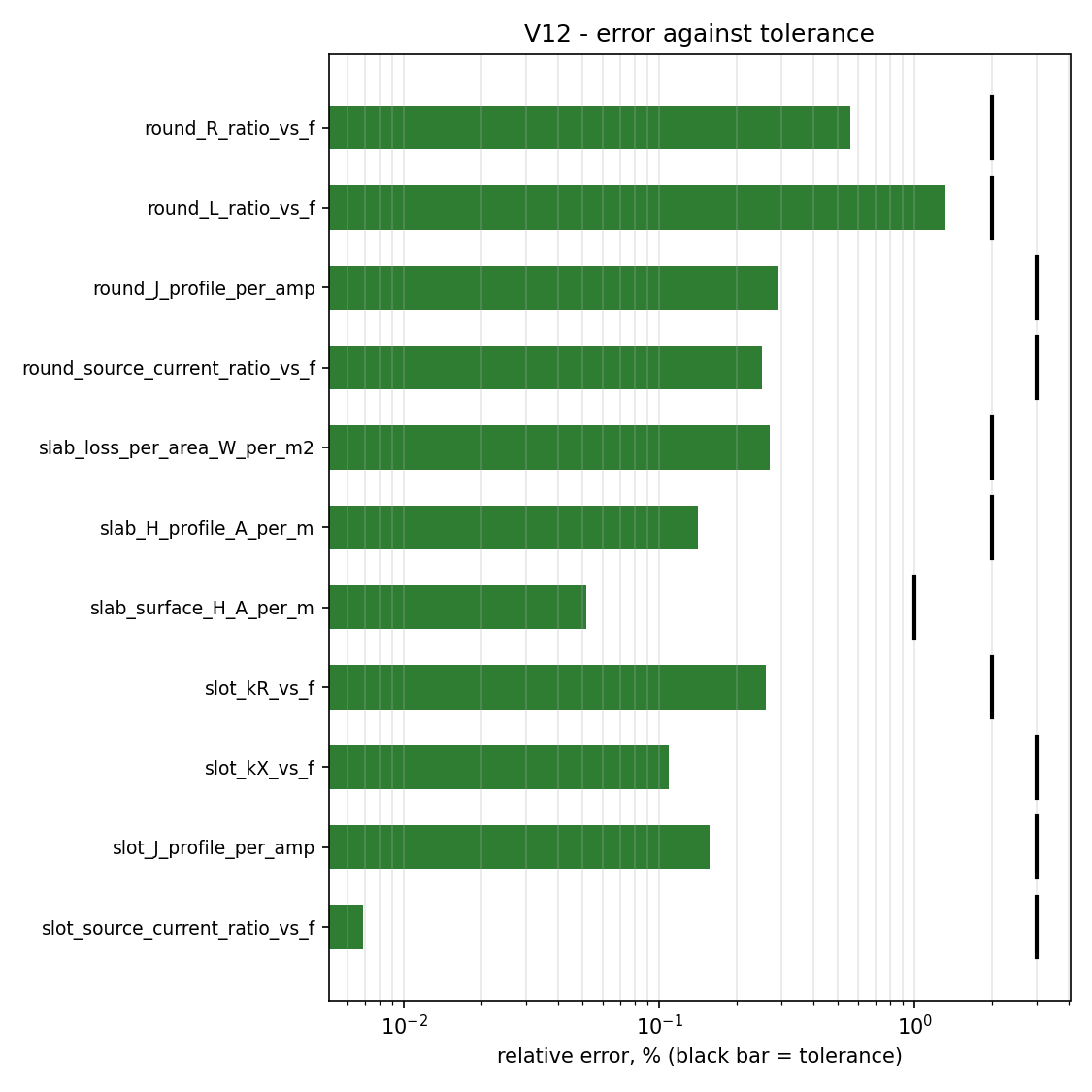
Every judged row passes, and the two that carry the plan's own tolerances pass with three to eight times the margin. R_ac/R_dc over five decades lands at +0.560 % (L2) against a 2 % tolerance, and Field's k_R — the deep-bar factor a machine designer actually uses — at +0.261 % across a range where the bar's resistance rises 6.8-fold. k_X is +0.108 % against 3 %. The slab's loss, which spans a factor of fifty across its three frequencies, is +0.271 %. The two current-density cuts reproduce their Bessel and cosh profiles to +0.292 % and +0.158 %, worst point +0.161 % of peak on a curve that spans a factor of three hundred.

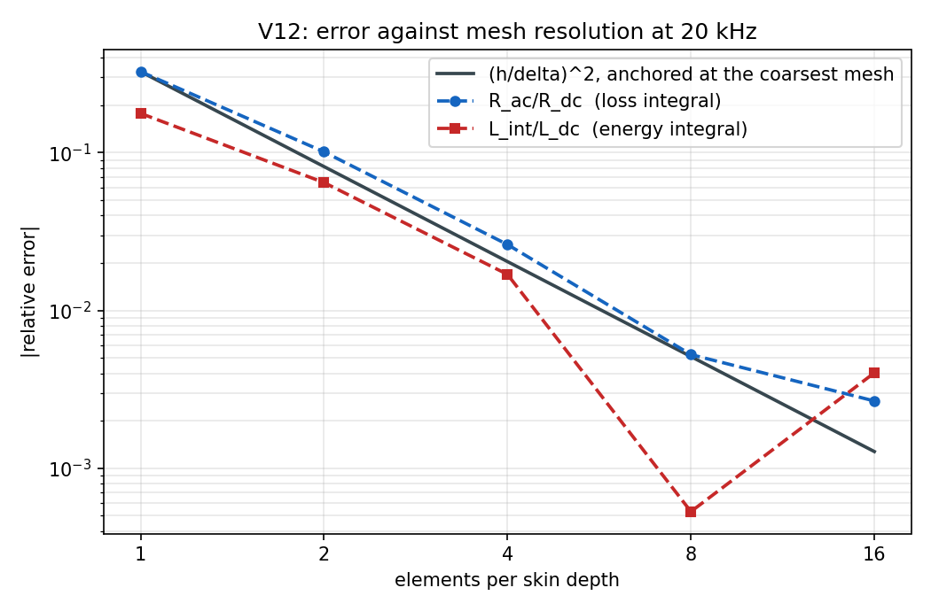
The mesh rule the plan states is not enough, and the case can say by how much. The validation plan asks for "≥ 4 elements per skin depth". Four resolves the field — the solution is smooth and P1 converges on it quadratically — but Nabla integrates a region's Joule loss from the nodal current density, and a node on a region boundary would otherwise average the conductor's J with the zero outside it. Results.populateFieldValues avoids that material blend by substituting the mean of the node's free neighbours inside the region — a value taken one element deep. Where J decays over a skin depth, that reads the surface layer low, and the surface layer is where the loss is. Measured, at 20 kHz:

Elements per skin depth	1	2	4	8	16
Error in R_ac/R_dc	−32.7 %	−10.1 %	−2.62 %	−0.53 %	+0.27 %

build.py predicted this before the run, as -2 (h/delta)^2, from the expansion of that substitution. The order is right and the coefficient is about five times too pessimistic: the fitted exponent is 1.98266, within 1 % of the predicted 2, while the measured error at four elements is -2.62 % rather than the −12 % the prediction gives. So the mechanism is established and the practical rule is one line: for a loss integral, resolve the skin depth with eight elements for 0.5 %, sixteen for 0.3 %. Four is enough for a field plot and would have failed this case's own 2 % tolerance.

The figure also shows where the sweep stops paying. The energy integral, drawn beside it as a control, reads the same solution through a path with no boundary substitution in it — and converges at the same order but crosses zero near eight elements, after which both curves sit on a floor of two to four parts in a thousand. That floor is the discretization of the model as a whole, and it is the number in the "16" column above.

The error budget of the round family closes to a tenth of a percent, and its largest term is the ammeter. The three lowest-frequency wire models share one mesh (the geometric floor binds, since a skin depth there is tens of millimetres) and all three report R_ac/R_dc +0.72 % and L_int/L_dc −1.58 %, where the exact answer at all three is 1. Neither is a skin-effect error — there is no skin effect at 2 Hz. Both follow from two mesh errors:

• the model's total current is measured from the slope of A in the air, and that reads 0.27 % low on the coarse air mesh (the round_source_current_ratio row, whose exact value is 1.0000 at these frequencies, comes out −0.27 %). Since R = P/I^2 and L = 2W/I^2, a current 0.27 % low is +0.54 % on both;
• the field-energy integral takes mean(B).mean(H) per element rather than mean(B.H), which is short by the within-element variance — about −2.1 % on a mesh with eight elements across the radius.

+0.54 and +0.54 - 2.11 are the two numbers observed. On the 20 kHz model, whose mesh is fifteen times finer, the ammeter error falls to −0.10 % and both rows fall with it, to +0.27 % and +0.40 %. Nothing here is unexplained, and nothing here is the eddy-current formulation.

What Nabla's harmonic drive actually is — and the case proves it rather than asserting it. The solver imposes a uniform J_src = I_src/S over a coil's region and adds the induced -j omega sigma A to it, with nothing constraining the sum to I_src. That is not an approximation of a current-driven conductor; it is exactly a voltage-driven one, since a uniform impressed current density is a uniform impressed E = J_src/sigma, i.e. a terminal voltage of I_src R_dc per metre. Two consequences, both tested:

1. The field is still exactly right. The constant particular solution A_p = J_src/(j omega sigma) cancels J_src identically, leaving J = -j omega sigma C J0(kr) — the correct profile at some total current. So every ratio judged here is untouched, provided the total current is measured rather than assumed. It is, from A in the current-free air outside.
2. The total current is predictable in closed form. Ohm's law for that voltage source gives I_total/I_src = R_dc/|Z_int + j omega L_ext|, and Nabla reproduces it to +0.253 % on the wire and +0.007 % on the slot — two geometries with nothing in common but the formulation. At 20 kHz the wire carries 3.9 % of its source current.

This matters to a user, and it is why the row is judged rather than filed as a curiosity: a solid conductor given a source current in a harmonic run does not carry that current. For a stranded winding — which is what a coil normally models, and what every machine case in this dossier uses — the impressed uniform density is correct and the question does not arise. For a bar, a busbar or a rotor cage driven directly rather than through a circuit, the delivered current must be read back. The case's reference notes §1.1 set out the algebra.

The slab's instrument row is the cheapest number in the case and the one that underwrites the rest of it. H at the slab surface reads +0.052 % of the I/L that Ampère's law makes exact, so the drive is delivering what the closed form assumes and the loss and profile rows are comparisons rather than coincidences.

6. Limitations

• Linear materials only. Every conductor here is copper with mu_r = 1, and the iron in the slot case is infinitely permeable, which is a boundary condition rather than a material. Skin effect in saturating steel — where the skin depth depends on the local field and the problem stops being a single frequency — is not tested by this case and has no closed form to test it against. V11's rotor steel is linear for the same reason.
• Time-harmonic only. Nothing here exercises the transient eddy-current path, which is a different assembly. V11 compares the two routes against each other at standstill and agrees to 0.9 %; this case does not repeat that.
• One conductor at a time. There is no proximity effect, no bundle, no transposition and no second conductor anywhere in the case. k_R for a multi-layer winding is a different (and much larger) number than the single-bar k_R measured here, and Field's formula for it is not tested.
• P1 only, planar only. The axisymmetric harmonic path and P2 harmonic kernels are not exercised; V09 and V17 own those.
• No circuit. Both driven families are excited by a coil's own AC source, not through the complex MNA. A conductor wired into a circuit takes a different route to its source term.
• The Jz probe blends materials at a region boundary. The judged cuts stop 0.1 a and 1 mm short of the surfaces for that reason. The region integrals do not have this problem — they carry the free-neighbour substitution discussed in §5 instead — so the limitation is on what a probe or a field plot shows at an interface, not on the numbers this case judges.
• The drive is a voltage source (§5). Every ratio in this chapter is normalised by the measured current and is therefore independent of that, but an absolute loss taken from a current-driven solid conductor is not.

7. Reproduce

cd validation
python -m harness.run_case V12

Requires a built triangle.exe (Nabla does not distribute it), a solver binary, and a licence carrying Core Pro (time-harmonic). Artifacts, including the sixteen models, land in cases/V12_skin_effect/artifacts/.

8. Changelog of the frozen reference

Date	Change	Reason
2026-08-11	case created; reference values and tolerances frozen before the case was run	the validation plan V12. The three tolerances the plan states (<= 2 % on R_ac/R_dc and k_R, <= 3 % on k_X, and the under-resolved run reported without a verdict) are transcribed verbatim. The rest are set from the physics and the discretization before any result existed: 2 % on the two integral sweeps that are the same kind of quantity as R_ac/R_dc, 3 % L2 / 5 % pointwise on the two current-density cuts because nodal Jz is a recovered element-constant field rather than the solution, 1 % on the slab's drive witness because it reads a slope of A in current-free air, and 3 % on the two source-current rows because their high-frequency end is dominated by an external inductance the air mesh has to represent. The MESH is not a tolerance and was chosen before the run from the error analysis written out in build.py: the plan's four elements per skin depth resolves the field but not the loss integral, whose boundary-node recovery carries an O((h/delta)^2) bias, so the judged sweeps use sixteen and the resolution sweep measures the curve. A smoke model of each of the three geometries was built first to establish the recipe - that the natural boundary is what models infinitely permeable iron, that the slab's mid-plane is A = 0, and that the total current has to be measured rather than assumed - and no tolerance was chosen from any of them.