V13 — Magnetized cylinder and far-field truncation study

← Back to the validation dossier

Tier A (analytic) - priority P0 Reference frozen on 2026-08-09. Nabla 0.1.0, solver licence mode enforcing, run in 50.3 s.

1. Problem

One permanent magnet, in free space, ten times.

A cylinder of radius a = 10 mm, uniformly magnetized transverse to its axis with remanence Br = 1.2 T and recoil permeability mu_r = 1, sits in air. Nothing else is in the model - no coil, no iron, no current anywhere. That is the point: this is the only case in the dossier whose entire excitation is the permanent-magnet source term, so nothing else can be credited for the answer.

The magnet is then solved with the outer boundary at R/a = 2, 3, 5, 10, 20, each radius terminated twice:

Sub-model	Outer boundary	Termination
dir2 .. dir20	2a, 3a, 5a, 10a, 20a	Dirichlet A = 0
ff2 .. ff20	the same five radii	far-field (balloon), BC type 11, decay order n = 1

Inside 2a every model is meshed by identical rules, so a difference between two sub-models is the boundary condition and not the mesh. The two terminations at a given radius are the same model differing in one BC record, and the mesh tables below confirm it: dir3 and ff3 have identical node and element counts.

The magnet's magnetization is the model input, M = Br/mu0 = 954.93 kA/m (ModelData holds a region's magnetization in kA/m). mu_r = 1 is deliberate - it is the textbook magnet, and it is what makes the interior answer exactly Br/2 instead of approximately it.

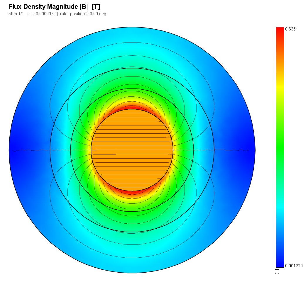
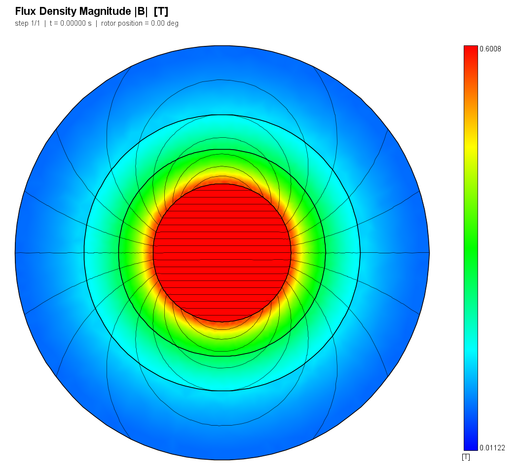
The two renders are the case in one picture, at the same radius, on the same mesh. On the left the outer boundary is a flux line, because A = 0 on it; every line has to turn and close inside the box, and the magnet works against the extra reluctance that costs. On the right the lines cross the boundary and carry on. (The colour scales are each render's own auto-scale, so read the lines, not the hues.)

2. Reference

Closed form throughout, derived in the case's reference notes and evaluated by harness/analytic.py at run time; a disagreement with the frozen numbers is reported as DRIFT and fails the case.

Inside the magnet the field is uniform, and outside it is an exact 2D dipole:

B_inside  = mu0 M / 2 = Br/2 = 0.6 T          H_inside = -M/2 = -477.46 kA/m
|B|(r)    = mu0 M a^2 / (2 r^2)               independent of angle
m         = pi a^2 M = 300 A*m per metre      (2D dipole moment)

H = -M/2 is the demagnetizing factor of a transversally magnetized cylinder, exactly 1/2, the two-dimensional companion of the sphere's 1/3.

The same two matching conditions also give the exact answer for a truncated model, and that is what makes this case more than a spot check:

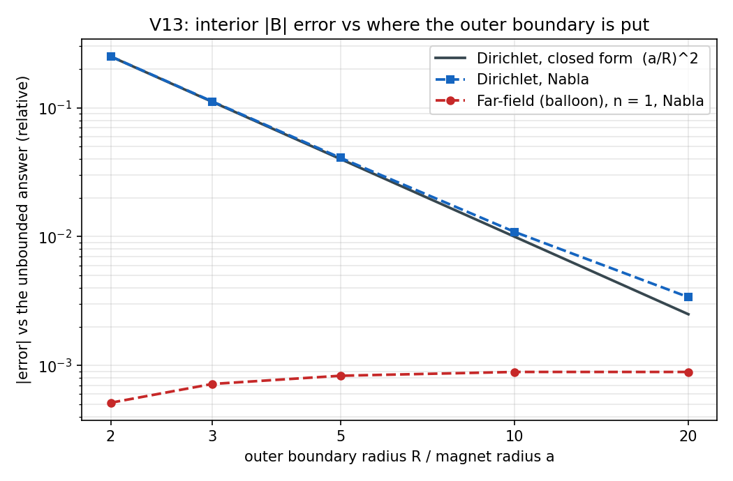
• a Dirichlet boundary at R adds an image term and lowers the interior field by exactly (a/R)^2 - -25.0 % at 2a, -11.1 % at 3a, -0.25 % at 20a;
• a first-order far-field boundary at R annihilates the growing term exactly: substituting the exterior expansion into dA/dr + A/R = 0 leaves 2 alpha = 0 and touches nothing else. For a source whose exterior field is a pure dipole, a balloon boundary is not an approximation at any radius.

So the Dirichlet leg is judged against the problem it really solved, the far-field leg against the unbounded problem, and every residual in either is discretization error. The harness proves the reference satisfies the balloon condition before the solver is asked about it (tests/test_harness.py::test_the_first_order_balloon_condition_is_exact_for_a_dipole).

Source statement as frozen: Closed form throughout. An infinitely long cylinder of radius a, uniformly magnetized transverse to its axis with magnetization M = Br/mu0 and recoil permeability mu_r = 1: inside, B = mu0M/2 uniform and H = -M/2 (the demagnetizing factor of a transverse cylinder is exactly 1/2); outside, an exact 2D dipole, |B| = mu0M*a^2/(2 r^2), isotropic in angle. The SAME two matching conditions give the exact answer for a model truncated by a Dirichlet A = 0 boundary at radius R, which lowers the interior field by exactly (a/R)^2 - so the Dirichlet leg of this case is judged against the problem it really solved, not only against the one it meant to. A first-order far-field (balloon) boundary annihilates the growing exterior term exactly for a dipole source, so the far-field leg is judged against the UNBOUNDED answer at every truncation radius. All of it is derived and evaluated in harness/analytic.py (section: uniformly magnetized cylinder); tolerances are transcribed from the validation plan, case V13.

3. Nabla model

Built entirely through nabla_api by build.py in this directory - no GUI step, no manual edit. Concentric circles at the magnet surface, at 1.5a and 2a, then geometric rings out to the boundary; each ring carries a maximum element area set from a target edge/radius ratio (0.05 inside 2a, 0.08 beyond), which is what keeps a 20a model roughly the price of a 3a one. Meshes for this run:

Sub-model	Element order	Nodes	Elements
dir2	P1	5009	9857
dir3	P1	5885	11674
dir5	P1	6833	13567
dir10	P1	7998	15904
dir20	P1	9371	18640
ff2	P1	5009	9857
ff3	P1	5885	11674
ff5	P1	6833	13567
ff10	P1	7998	15904
ff20	P1	9371	18640

Every sub-model is P1 and comfortably under the free tier's 25 000-node cap, but this case is not reproducible on the free tier: the far-field boundary condition is a Core Pro feature and assignBC(11, ...) refuses without it. The Dirichlet half runs unlicensed. The models are published beside this chapter under artifacts/models/.

4. Results

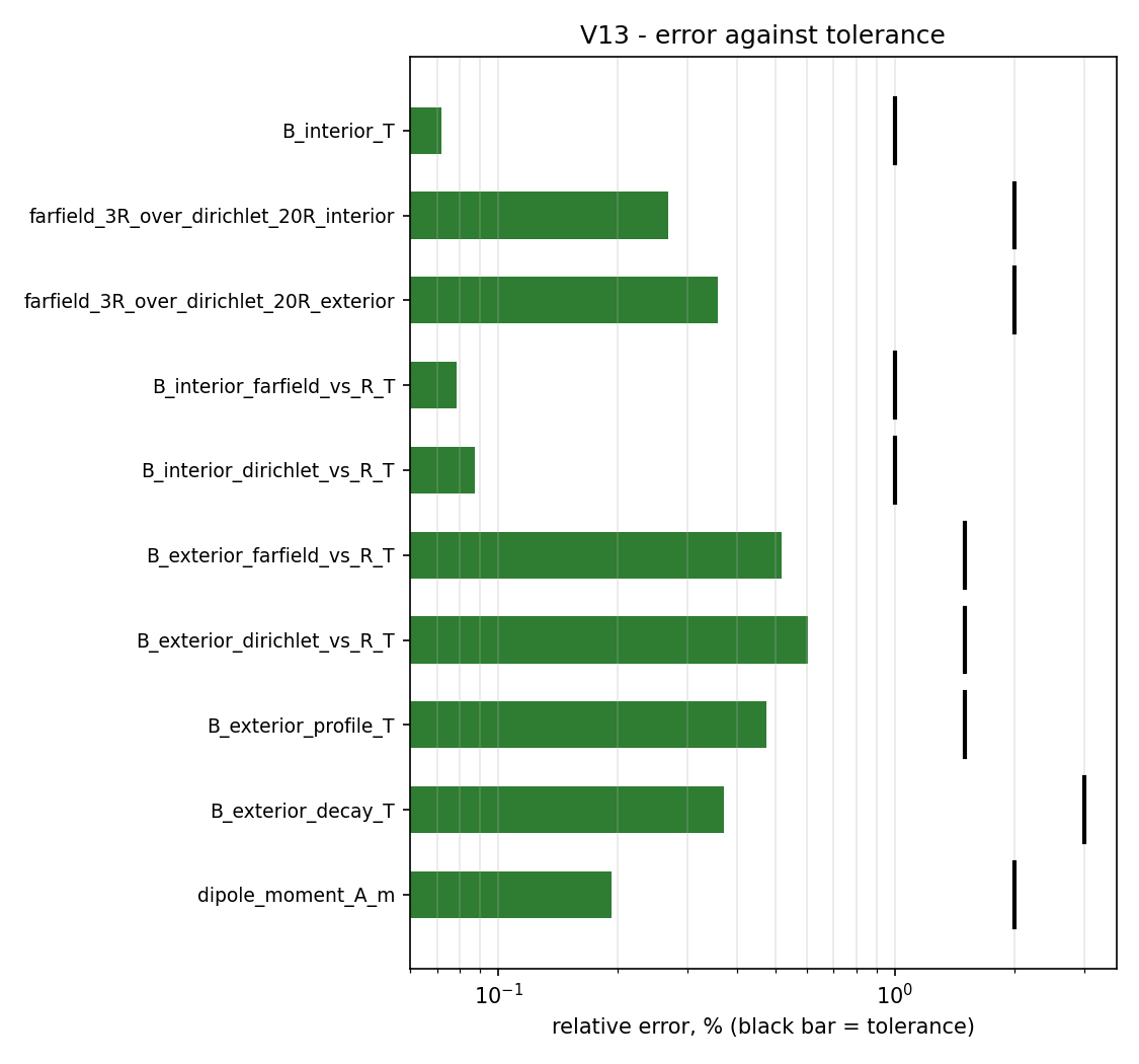
Quantity	Metric	Nabla	Reference	Error	Tolerance	Verdict
B_interior_T	rel	0.599568 T	0.6 T	-0.072 %	1.000 %	PASS
farfield_3R_over_dirichlet_20R_interior	rel	1.00268 -	1 -	+0.268 %	2.000 %	PASS
farfield_3R_over_dirichlet_20R_exterior	rel	1.00358 -	1 -	+0.358 %	2.000 %	PASS
B_interior_farfield_vs_R_T	profile	min=0.5995, max=0.5997, rms=0.5995 T	min=0.6, max=0.6, rms=0.6 T	L2 +0.078 %, max +0.089 %	L2 1.000 %, max 1.500 %	PASS
B_interior_dirichlet_vs_R_T	profile	min=0.4497, max=0.598, rms=0.5526 T	min=0.45, max=0.5985, rms=0.5531 T	L2 +0.087 %, max +0.090 %	L2 1.000 %, max 1.500 %	PASS
B_exterior_farfield_vs_R_T	profile	min=0.3041, max=0.3078, rms=0.3062 T	min=0.3061, max=0.3061, rms=0.3061 T	L2 +0.517 %, max +0.661 %	L2 1.500 %, max 2.500 %	PASS
B_exterior_dirichlet_vs_R_T	profile	min=0.1541, max=0.3063, rms=0.2626 T	min=0.1561, max=0.3046, rms=0.2624 T	L2 +0.604 %, max +0.672 %	L2 1.500 %, max 2.500 %	PASS
B_exterior_profile_T	profile	min=0.1573, max=0.4508, rms=0.2812 T	min=0.1578, max=0.4537, rms=0.2817 T	L2 +0.475 %, max +0.642 %	L2 1.500 %, max 3.000 %	PASS
B_exterior_decay_T	profile	min=0.002648, max=0.4153, rms=0.1547 T	min=0.002667, max=0.4167, rms=0.1552 T	L2 +0.370 %, max +0.326 %	L2 3.000 %, max 6.000 %	PASS
dipole_moment_A_m	rel	299.421 A*m	300 A*m	-0.193 %	2.000 %	PASS
B_interior_uniformity_rel	abs	8.28466e-06 -	0 -	8.285e-06	0.01	PASS
B_exterior_isotropy_rel	abs	0.00938646 -	0 -	0.009386	0.02	PASS
H_interior_x_A_per_m	rel	477039 A/m	-477465 A/m	+199.911 %	-	REPORT
dirichlet_3R_error_vs_open_rel	rel	-0.111881 -	-0.111111 -	-0.693 %	-	REPORT

5. Discussion

The permanent-magnet source term is right. Interior |B| lands at -0.072 % of Br/2, and across five interior stations it varies by a fraction 8.28466e-06 of its own mean - eight parts in a million, so the equivalent surface-current formulation leaves no gradient behind inside the magnet. The exterior field follows the dipole law to +0.475 % (L2) over the near cut and +0.370 % out to 15a, across more than two decades in |B|. Around a circle at 1.4a, where the exact |B| is independent of angle, it varies by a fraction 0.00938646 of its mean - under 1 %, and that is the mesh's own anisotropy, since the reference has none. Fitting the exterior field back to a source returns a dipole moment of 299.421 A*m against the exact 300 - a round trip from magnetization to field and back that closes to -0.193 %.

The truncation figure is the case. The Dirichlet curve sits on the closed form (a/R)^2 across two decades of nothing-but-boundary-error, from -25 % at 2a to -0.25 % at 20a, and Nabla reproduces that closed form to +0.087 % - the box is wrong and the solver is right about how wrong. The far-field curve is flat between 0.05 % and 0.09 %, at every radius including 2a, and that band is the discretization floor of this mesh rather than a boundary error: the balloon boundary has removed the truncation error entirely rather than reduced it. Note where the two curves meet the floor - by 20a even the Dirichlet run is down at 0.34 %, which is why 20x is the number the folklore quotes, and the point of the far-field condition is that it is already there at 2x.

The claim in the far-field boundary specification, in one row. Far-field at 3a against Dirichlet at 20a agrees to +0.268 % inside the magnet and +0.358 % at the exterior station, against a 2 % tolerance. The residual has a known sign and a known size: the exact ratios are 1.00251 and 1.00492, because a Dirichlet box at 20a is itself 0.25 % and 0.49 % short. The balloon answer is the better of the two, and the "reference" it is being held to is the approximation. The other half of the claim is the row published without a verdict: a Dirichlet box at 3a comes out -0.111881 relative to the unbounded answer - an 11 % error a user would have no way of noticing, because a converged-looking solve on a perfectly good mesh returns it without complaint.

Where the remaining error is. The interior probes are flat to better than 0.05 % across all ten models; the exterior station scatters by about ±0.6 % between radii, and that scatter is the mesh, not the boundary. It can be seen directly: at each radius the Dirichlet and far-field errors track each other - +0.43 % / +0.54 % at 3a, +0.32 % / +0.35 % at 5a, -0.54 % / -0.55 % at 10a, +0.56 % / +0.57 % at 20a - because the pair shares a mesh exactly. What differs between the two columns is the physics; what they share is the recovery error of nodal B in a 1/r^2 field, which is O((h/r)^2) and does not care which BC produced the solution.

One finding ships without a verdict, and it is not about the boundary. H probed at the centre of the magnet reads 477039 A/m where the exact answer is -477465 A/m: the right magnitude and the wrong sign. What the solver exports as H is B/(mu0 mu_r), with no -M term, so inside a magnet region it is not the magnetic field strength - it is B divided by a permeability. Outside magnets it is correct and nothing else in this case or any other is affected, because the field solution itself is unaffected: the magnetization enters the source vector, not the constitutive read-back. But an engineer who opens the H plot to check whether a magnet is being demagnetized will read a large positive H along M and conclude the opposite of the truth. Nabla's own demagnetization assessment does not go through this path - the Demag Risk field evaluates B . m_hat against the material's demagnetization curve, and the eggshell force integral applies the full B = mu(H + M) law - so this is a display and probe defect rather than a wrong answer anywhere. It is recorded here because a validation case that noticed it and did not say so would be worth less than one that never ran.

6. Limitations

• This proves the PM source term, not PM materials. The magnet is linear with mu_r = 1 and a prescribed magnetization. It is not a catalogue material, there is no demagnetization curve, no knee, no temperature, and no irreversible loss. The magnetic materials reference and the Demag Risk post-processing are not exercised here.
• The balloon result is exact because the source is a dipole. n = 1 is the correct decay order for this problem, so the boundary condition is not merely accurate but exact, and the flat error curve should not be read as a promise for other geometries. The far-field boundary specification §4b measures the price of a wrong n (a factor of ~45 at R = 3a for a dipole source), and a machine cross-section needs n = p. What this case establishes is that the implementation delivers the exact answer where the exact answer is known.
• A net current is out of scope. No r^-n asymptotic condition can represent the ln r exterior of a model carrying net current; the model here carries none. Nabla's checklist warns about it and this case does not test it.
• Planar 2D, static, P1, linear, no motion. The axisymmetric far-field variant is measured in the far-field boundary specification §4b Phase 4 and is picked up by V17.
• The exterior probes read nodal B, which is averaged over the elements around a node; that is why every exterior station is placed at least ten elements clear of the magnet surface, where a nodal average would blend two materials.

7. Reproduce

cd validation
python -m harness.run_case V13

Requires a built triangle.exe (Nabla does not distribute it), a solver binary, and a licence carrying Core Pro for the five far-field sub-models. Artifacts, including the ten models, land in cases/V13_magnetized_cylinder/artifacts/.

8. Changelog of the frozen reference

Date	Change	Reason
2026-08-09	case created; reference values and tolerances frozen before the case was run	the validation plan V13. The four tolerances the plan states (interior B <= 1 %, far-field at 3R within 2 % of the 20R Dirichlet reference) are transcribed verbatim. The rest are set from the physics before any result existed: 1-1.5 % where the probe sits in the fine near mesh shared by every sub-model, 3 % on the long-range decay cut whose air is deliberately graded at h = 0.08 r. A smoke model at R = 3a was built first to establish the model recipe - that a region's magnetization is held in kA/m, that DOM = 0 points along +x, and that the boundary condition must be assigned before the circles are subdivided - and no tolerance was chosen from it.