V15 — Force methods cross-check on a linear actuator

← Back to the validation dossier

Tier A+S (analytic + self-consistent: method equivalence) - priority P1 Reference frozen on 2026-08-13. Nabla 0.1.0, solver licence mode enforcing, run in 72.7 s.

1. Problem

One actuator, asked for its force three different ways, at twelve plunger positions.

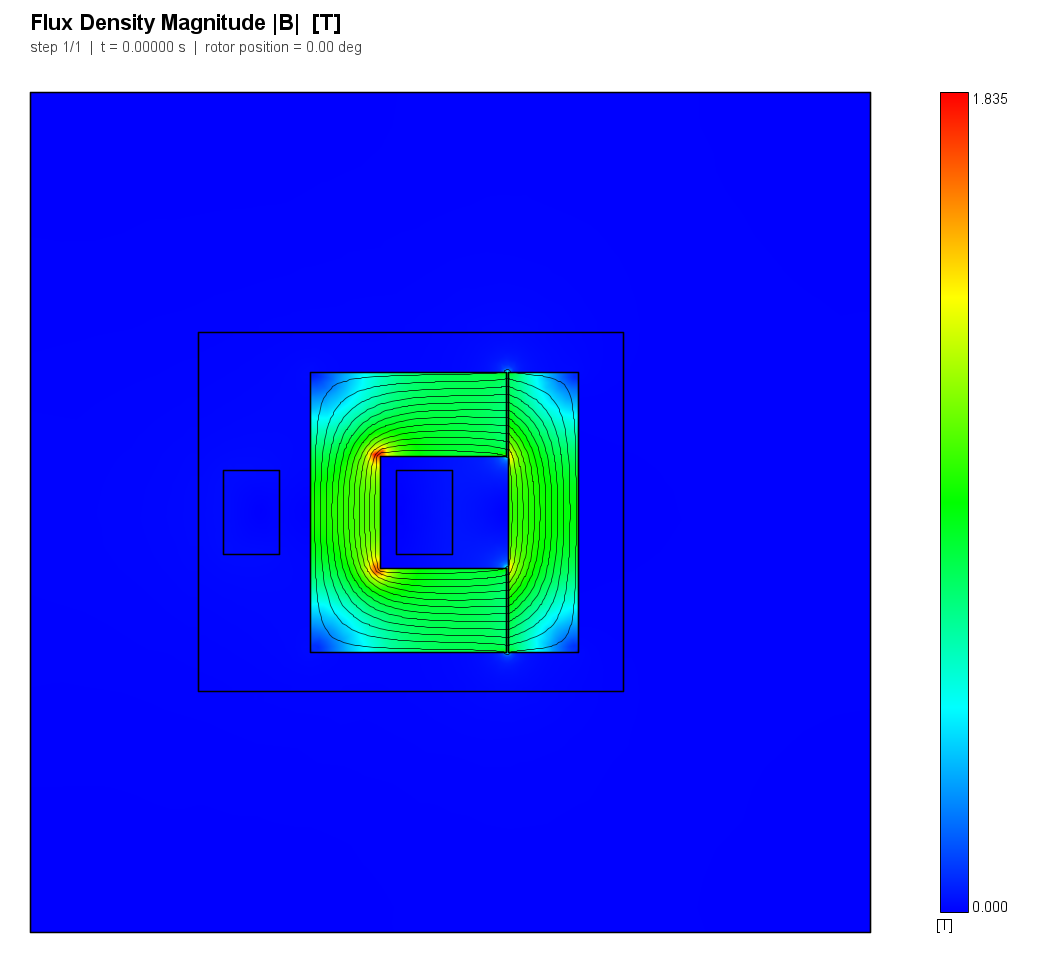
A wound C-core faces a movable iron plunger across two airgaps. The coil carries 400 turns at 3 A - 1200 ampere-turns, held constant - and the plunger is swept from 0.4 mm to 2.6 mm in 0.2 mm steps, over which the pull falls from 3.74 kN to 120 N, a factor of 31. A thirteenth solve repeats the 1.0 mm position with the plunger cut into two touching iron regions.

Core	70 x 100 mm, 25 mm back leg, two 30 mm pole faces, window 45 x 40 mm
Plunger	25 mm thick, full core height, at x = 70 + gap
Iron	linear, mu_r = 2000, both bodies
Coil	400 turns, 3 A DC, go inside the window and return outside the core
Depth	60 mm, planar 2D, P1, static
Sweep	gap = 0.4 ... 2.6 mm in 0.2 mm steps (12 positions)
split	the same model at 1.0 mm, plunger cut into a 10 mm face piece and a 15 mm back piece

The iron is linear on purpose, and that is a design decision rather than a convenience. The virtual-work force is the derivative of the coenergy W_co = INT H B.dH, and what Nabla's region post-processing returns is the energy W = INT B H.dB (FEMM's block integral 2). The two are the same number only for a linear, unmagnetized material. A nonlinear sweep would need a coenergy read-back no API exposes, and would have tested the BH curve - which V02 does - instead of the three force methods, which is what this case is for.

The three methods. They share the solution and nothing else:

• eggshell - getResultsInRegion(region, "Force"), the weighted Maxwell stress integral over the one-element shell around the region, evaluated with the Korteweg-Helmholtz (coenergy) tensor, reading element B and the element's own material;
• contour - addProbeContour + getForce, the vacuum Maxwell stress integrated over a closed contour this case draws itself in air, reading nodal B and nodal mu at 1000 sampling stations;
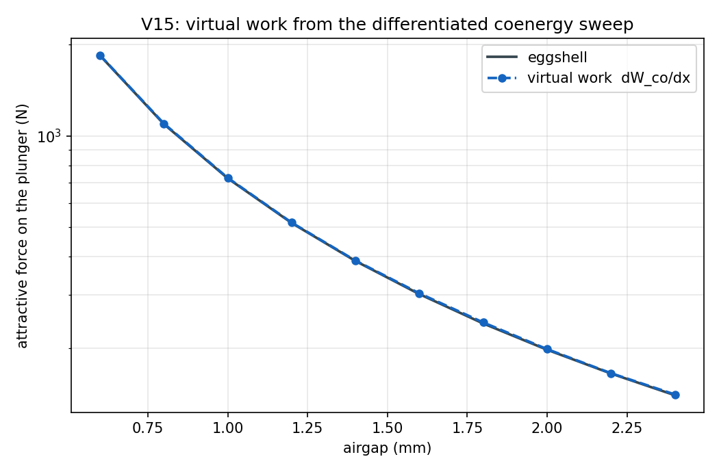
• virtual work - -dW_co/dx at constant current, differenced across the position sweep, reading no field at all - only the summed region field energy.

Three post-processors, three field read-backs, one force. If the number they return depends on which one is asked, at least two of them are wrong.

2. Reference

Derived in full in the case's reference notes. Two things, one of them a formula and four of them identities.

The closed form. For a gap short compared with the pole face, the field in it is uniform and normal, and the Maxwell stress is a pure tension:

F = B^2 A / (2 mu0)      per gap,   two gaps in this circuit

B is the flux density the solution reports over the pole face (the mean of |Bx| over 40 midpoint stations on each face, at mid-gap); the closed form supplies only the step from that flux density to a force, and that step is what is judged. Its neglected term is fringing - flux that leaves the pole outside the face and still pulls - which in a planar model is O(gap / pole width) and is positive in the force. The case therefore judges it only where gap/width <= 0.02, which is fixed in geometry.json and covers the 0.4 and 0.6 mm positions, and publishes the ratio at all twelve.

The identities. Two surfaces enclosing the same body in air must return the same force, because the vacuum stress tensor is divergence-free in current-free air. Virtual work must return it a third time. And two touching parts of one body must sum to the force on the body - the split between them is a stress-model convention (the force-calculation specification §2), the sum is not. Every one of those references is exactly 1.0, and the tolerances - 2 % pairwise, 3 % on the closed form in its window, 1 % on additivity - are transcribed verbatim from the validation plan V15.

Source statement as frozen: Two references, both exact. (1) The pull of one airgap on an idealized C-shaped actuator, F = B^2 A / (2 mu0) per gap, where B is the flux density the solution reports over the pole face and A is the face area: this is the Maxwell stress of a uniform normal field, and it is exact in the unsaturated small-gap limit and nothing else. Its leading correction is fringing, O(gap / pole width), so it is JUDGED only where that ratio is <= 0.02 (gaps 0.4 and 0.6 mm on a 30 mm pole face) and the ratio is published at every position so the reader sees the closed form leave its own window. (2) Every other judged row is an identity rather than a number: three methods that measure the same force must return the same force (Maxwell stress on a contour, the eggshell region integral, and virtual work from the differentiated coenergy sweep), and the forces on two touching parts of one body must sum to the force on the body (the force-calculation specification section 2 - the pair invariant is unique even where the split between the parts is a modelling convention). Those rows have reference exactly 1.0. Tolerances are transcribed verbatim from the validation plan, case V15: pairwise agreement of the three methods <= 2 %, the closed form in its validity window <= 3 %, additivity <= 1 %.

3. Nabla model

Built entirely through nabla_api by build.py in this directory - no GUI step, no manual edit, every dimension from geometry.json. Meshes for this run:

Sub-model	Element order	Nodes	Elements
g04	P1	14486	28875
g06	P1	11727	23356
g08	P1	10231	20366
g10	P1	9430	18755
g12	P1	8758	17417
g14	P1	8319	16540
g16	P1	7998	15898
g18	P1	7759	15422
g20	P1	7615	15132
g22	P1	7398	14695
g24	P1	7237	14378
g26	P1	7201	14304
split	P1	9385	18677

Two mesh rules carry the case, and both were fixed before the first solve:

• Six element layers across every gap. The gap-facing boundaries of both irons are subdivided to min(gap/6, 0.5) mm, so the mid-gap stress contour stands three element layers clear of each iron surface. Three, not one, because the contour probe reads nodal B and nodal mu, which are averaged over every element sharing the node and are therefore contaminated within one layer of a material interface (case V21 finding F1). V02 measured the price of getting this wrong: a contour standing 5 mm off a body in 6 mm air disagreed with the eggshell by 3.5 %.
• A refined air box around the whole device, meshed at 2.5 mm rather than the far-field 15 mm, so that the widest contour in the clearance sweep - 9 mm off the plunger - is still several element layers out in properly resolved air.

The contour itself runs up the middle of each airgap where a pole faces the plunger (there is nowhere else for it to go at 0.4 mm) and stands one clearance off every other iron surface, dipping into the window air between the poles with its corners held one clearance clear of the core's window faces, so that no stretch of it ever runs along an interface. It is evaluated at three clearances - 3, 6 and 9 mm - on every solution.

The models are published beside this chapter under artifacts/models/.

4. Results

Quantity	Metric	Nabla	Reference	Error	Tolerance	Verdict
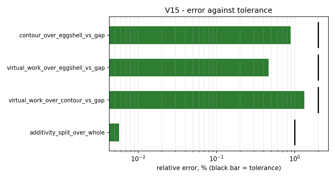
contour_over_eggshell_vs_gap	profile	min=0.9872, max=0.9969, rms=0.9918 -	min=1, max=1, rms=1 -	L2 +0.888 %, max +1.283 %	L2 2.000 %, max 2.000 %	PASS
virtual_work_over_eggshell_vs_gap	profile	min=1.002, max=1.008, rms=1.004 -	min=1, max=1, rms=1 -	L2 +0.462 %, max +0.805 %	L2 2.000 %, max 2.000 %	PASS
virtual_work_over_contour_vs_gap	profile	min=1.006, max=1.018, rms=1.013 -	min=1, max=1, rms=1 -	L2 +1.321 %, max +1.817 %	L2 2.000 %, max 2.000 %	PASS
closed_form_over_eggshell_small_gap	profile	min=0.9835, max=0.9889, rms=0.9862 -	min=1, max=1, rms=1 -	L2 +1.405 %, max +1.648 %	L2 -, max 3.000 %	PASS
additivity_split_over_whole	rel	0.999943 -	1 -	-0.006 %	1.000 %	PASS
closed_form_over_eggshell_vs_gap	profile	min=0.9309, max=0.9889, rms=0.9595 -	min=1, max=1, rms=1 -	L2 +4.459 %, max +6.908 %	L2 -, max -	REPORT
virtual_work_raw_over_reciprocal_vs_gap	profile	min=1.005, max=1.097, rms=1.028 -	min=1, max=1, rms=1 -	L2 +3.863 %, max +9.731 %	L2 -, max -	REPORT
virtual_work_flux_linkage_over_energy_vs_gap	profile	min=1, max=1, rms=1 -	min=1, max=1, rms=1 -	L2 +0.000 %, max +0.000 %	L2 -, max -	REPORT
contour_clearance_spread_max	abs	0.00873803 -	0 -	0.008738	-	REPORT
additivity_contour_split_over_whole	rel	1.00207 -	1 -	+0.207 %	-	REPORT
split_front_force_share	rel	1.00074 -	1 -	+0.074 %	-	REPORT
b_face_over_reluctance_nominal	rel	0.99781 -	1 -	-0.219 %	-	REPORT
force_over_reluctance_nominal	rel	0.990553 -	1 -	-0.945 %	-	REPORT
b_face_vs_gap_T	report	(series)	-	-	-	REPORT
coenergy_vs_gap_J	report	(series)	-	-	-	REPORT
force_pull_closed_form_vs_gap_N	report	(series)	-	-	-	REPORT
force_pull_contour_vs_gap_N	report	(series)	-	-	-	REPORT
force_pull_eggshell_vs_gap_N	report	(series)	-	-	-	REPORT
force_pull_virtual_work_vs_gap_N	report	(series)	-	-	-	REPORT

• b_face_vs_gap_T: extracted but not frozen in expected.json - reported only
• coenergy_vs_gap_J: extracted but not frozen in expected.json - reported only
• force_pull_closed_form_vs_gap_N: extracted but not frozen in expected.json - reported only
• force_pull_contour_vs_gap_N: extracted but not frozen in expected.json - reported only
• force_pull_eggshell_vs_gap_N: extracted but not frozen in expected.json - reported only
• force_pull_virtual_work_vs_gap_N: extracted but not frozen in expected.json - reported only

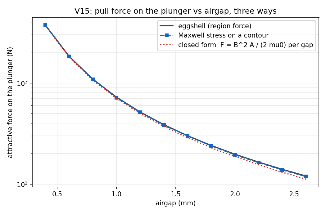
5. Discussion

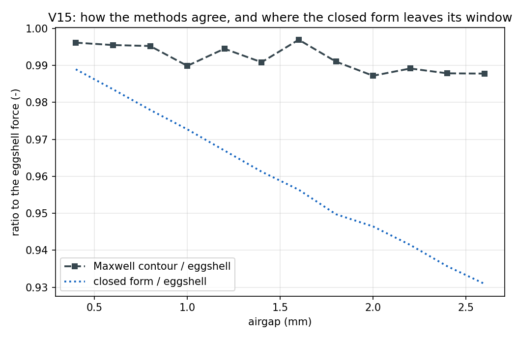
The three methods agree, and the widest disagreement anywhere is 1.8 %. Across twelve plunger positions and a 31-fold range in force, the contour integral sits +0.888 % (L2, unsigned) below the eggshell force with a worst point at +1.283 %, and virtual work sits +0.462 % above it, worst point +0.805 %. The ordering is consistent rather than random - contour below, eggshell in the middle, virtual work above - which is why the third pairing is reported separately: agreement is not transitive at a tolerance, and contour against virtual work is +1.321 %, the largest of the three and still inside 2 %.

The two Maxwell-stress surfaces differ because they read the field differently. The eggshell uses element B and each element's own material; the contour probe interpolates nodal B and nodal mu at 1000 stations, and nodal recovery on P1 elements is an averaging operation with its own O(h²) error. The contour's deficit does not grow as the contour moves: over clearances of 3, 6 and 9 mm the force changes by at most +0.87 % of itself, which says the contour is not sampling a contaminated first element layer anywhere - it is reading a slightly smoothed field everywhere. That is the number V02's chapter asked for and could not produce from a single contour.

Virtual work is the row worth pausing on, because it shares nothing with the other two but the solution vector. No stress tensor, no surface, no probe: twelve independent solves, their total field energy, and a derivative. It lands within 0.81 % of a surface integral of the field at every position. Two things had to be right at once for that: the region energy integral (element B through each element's own material - the path case V21 finding F1 established) and the sensitivity of the whole solution to a 0.2 mm change in geometry.

The differencing scheme is declared, and it earns its keep. W(g) for a magnetic circuit is a hyperbola, so a plain central difference carries an (dg/g)² truncation error; the difference is therefore taken on 1/W, which is a straight line, and the naive result is published beside it. It comes out +9.731 % high at the smallest differenced position and falls off exactly as the law predicts - 9.7 % measured against 11.1 % predicted at 0.6 mm, 3.6 % against 4.0 % at 1.0 mm, 0.55 % against 0.69 % at 2.4 mm, tracking (dg/g)² to about 0.87 of it across the sweep (the shortfall is the iron's own reluctance, worth 0.07 mm of airgap, plus the leakage energy the hyperbola omits). Had the naive difference been used, the virtual-work row would have failed its 2 % tolerance at five of the ten positions - and it would have been the scheme failing, not the solver. Stating it in advance is what separates the two.

The closed form leaves its window on a straight line. Inside the window its worst point deviates by +1.648 %, and it is a deficit: the fringing the formula omits, with the sign fringing must have. Outside, the deficit grows to 6.9 % by 2.6 mm, and across the whole sweep it is 1 - F_ideal/F = 0.82 (gap/width) to within ±0.02 in the coefficient - a straight line over a 6.5-fold range in gap and a 31-fold range in force. This is the case's most quotable engineering result: a hand calculation from the pole-face flux density is good to about 0.8 g/w, so at g/w = 1/100 it is a 1 % answer and at g/w = 1/10 it is an 8 % one, and it is always an underestimate.

The pair invariant holds to six parts in a hundred thousand. Cutting the plunger into two touching iron regions and adding their forces reproduces the one-region result to -0.006 % against a 1 % tolerance. That is the check the force-calculation specification §2 asks for, and it is the one that makes Nabla's Korteweg-Helmholtz force on a region not surrounded by air trustworthy: the shell around the front piece runs through solid iron, where a vacuum stress tensor would return an arbitrary shell-position-dependent number. The control row says how much of that agreement is luck: the contour force - which lies in air and never sees the internal cut - differs between the two models by +0.207 %, so the two meshes are worth about 0.2 %, and the additivity agreement is a factor of thirty better than the mesh noise it is measured through. The split itself is a stress-model convention and is published as one: the 10 mm face piece is attributed 1.00074 of the total, i.e. the back piece carries a slight negative share, which is what a coenergy tensor does when the flux has already turned by the time it reaches the interface.

The lumped model, without a verdict. The reluctance sketch with a planar fringing correction predicts the pole-face flux density at the nominal gap to -0.219 % and the force to -0.945 %. That is closer than a hand model deserves to be, and it should not be read as a general result - this actuator is a short, fat, low-leakage circuit running at about 0.70 T through both the gap and the core legs, on linear iron. That is the best case a reluctance model will ever see. V02 makes the same point from the other end, where the iron saturates.

One free identity worth naming. Taking the virtual-work derivative on the coil's flux linkage (W = 0.5 lambda I) instead of on the summed region energy reproduces it to +0.000 % - six parts in 10^12. That is not independent physics: for a linear system the discrete identity 0.5 A^T K A = 0.5 lambda I holds exactly in the finite element algebra. It is published because it is a genuine check on the two post-processors having implemented what they claim, and because a reader who saw the row without this note would over-credit it.

6. Limitations

• Linear iron. Nothing here exercises the BH curve, and the equality of energy and coenergy that the virtual-work leg rests on is a consequence of that choice. A nonlinear virtual-work check needs a coenergy read-back Nabla does not currently expose through the API; until it does, the nonlinear force is covered by the eggshell-versus-FEMM comparison in V02 and by the KH tensor's own coenergy tables, which are exercised but not separately validated here.
• Planar 2D, static, P1, no motion. The axisymmetric force (F_z on an axisymmetric eggshell) and the P2 force integrals are not tested. Note in particular that the contour force path is planar-only - it multiplies by the model axial length rather than by 2 pi r - so an axisymmetric contour force is out of scope here and should be treated as untested.
• A single geometry class. A C-core pulling a flat armature has its force overwhelmingly in two well-behaved parallel-faced gaps. It says nothing about a force that comes from a tangential field, from a corner, or from a body with no facing pole; the tangential (torque) case is V04, V05 and V11's subject, and V05 records that a single-contour stress integral is the wrong tool there.
• The outer boundary is a Dirichlet box roughly one device-size out, which suppresses a little of the leakage flux. That is deliberate and harmless here: all three methods read the same truncated solution, and the closed form is fed the same solution's own gap flux density, so no judged row of this case is sensitive to it. The absolute forces in the artifacts should not be quoted as the forces of an unbounded actuator.
• No absolute force is judged. Every judged row is a ratio, plus the closed form in its window. The case proves the force post-processors against each other and against the physics; that the field they read is itself right is V01, V02 and V13's job.
• 1000 contour sampling stations is the default and was not swept. The clearance sweep bounds the contour's sensitivity to placement, not to sampling density.

7. Reproduce

cd validation
python -m harness.run_case V15

Requires a built triangle.exe (Nabla does not distribute it) and a solver binary. No gated feature is used, so the case runs on the free tier as long as the meshes stay under its 25 000-node cap - the largest here is at 0.4 mm and well inside it. Artifacts, including the thirteen models, land in cases/V15_force_methods/artifacts/.

8. Changelog of the frozen reference

Date	Change	Reason
2026-08-13	case created; reference values and tolerances frozen before the case was run	the validation plan V15. All three tolerances (pairwise 2 %, closed form 3 %, additivity 1 %) are transcribed verbatim from the plan. Everything the case chose for itself was chosen from the physics before any result existed: the pole face is 30 mm wide and the sweep starts at 0.4 mm so that the closed form has a validity window inside the sweep (gap/width = 0.013); the gap ladder is uniform at 0.2 mm because the virtual-work leg central-differences it; the mesh puts six element layers across every gap so that the mid-gap stress contour is three layers clear of both irons, from case V21 finding F1 and V02's contour finding; and the coenergy difference is taken on 1/W, whose leading truncation term vanishes for a magnetic circuit, with the naive difference published beside it. The iron is linear so that the region Field Energy read-back IS the coenergy the virtual-work identity needs.