V16 — Transformer: magnetizing and short-circuit impedance

← Back to the validation dossier

Tier A + X (analytic + cross-code) - priority P1 Reference frozen on 2026-08-15. Nabla 0.1.0, solver licence mode enforcing, run in 1223.3 s.

1. Problem

A two-winding transformer, seven times.

Two concentric windings sit on one limb: an inner LV winding of 100 turns and an outer HV winding of 400, separated by a gap, with a duct between the limb and the LV winding. Rated ampere-turns are 12 000 on each. Everything the case compares is referred to the HV winding, at 50 Hz.

Sub-model	Formulation	Excitation	What it is for
window_planar	planar, static, linear	balanced ampere-turns	the classical window, where the closed form is EXACT
window_axi	axisymmetric, static, linear	balanced	the same window revolved: the true concentric geometry
window_harmonic	planar, time-harmonic 50 Hz	balanced, AC	the rated-frequency run must return the static answer
sc_core	planar, static, linear iron	balanced	a real closed core, window taller than the windings
oc_linear	planar, static, linear iron	HV alone	magnetizing inductance, turns-ratio transfer
oc_saturated	planar, transient, M-36 steel, circuit-coupled, Crank-Nicolson	HV from a voltage source	the magnetizing current, and its distortion
oc_saturated_be	the same, Backward Euler, one period	the same	one row: what a first-order scheme does to a driven flux

The short circuit is imposed as balanced ampere-turns rather than as a shorted secondary. The two differ by the magnetizing current, which oc_linear measures at 0.000286221 per unit; the balanced pair is what every closed form in the literature is written for, and it removes the circuit solver from a measurement that is about the leakage field. The circuit coupling is not skipped, it is put where it matters: oc_saturated is fed from a stiff sinusoidal voltage source, which is the only way to get a sinusoidal flux and therefore the peaked magnetizing current this chapter ends on.

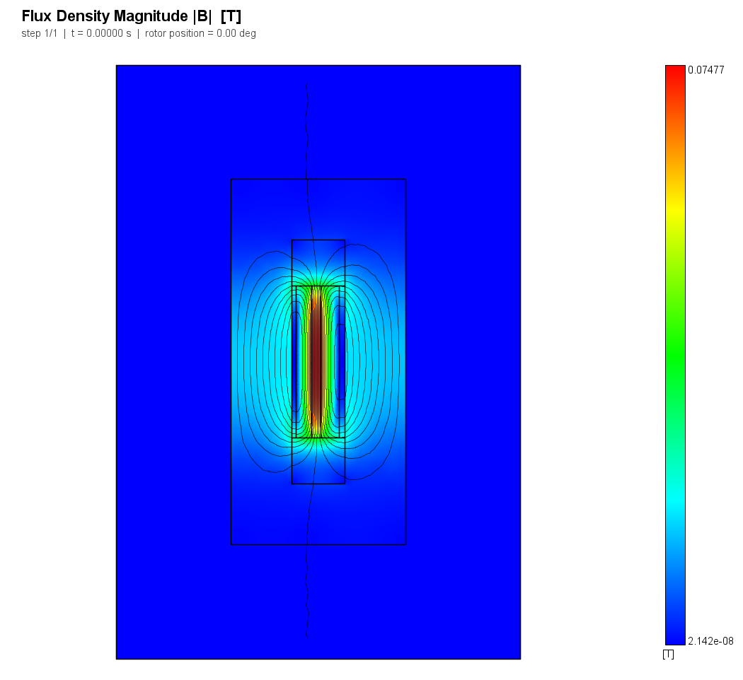
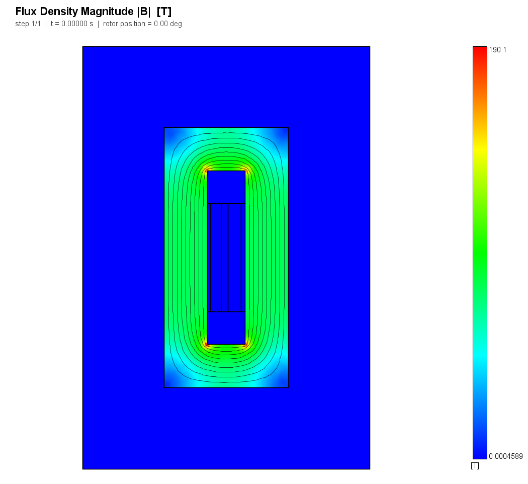
Two pictures of the same model differing only in what the LV winding is doing. On the left the ampere-turns balance and every flux line is trapped in the window, running axially between the two windings - that field, and only that field, is the short-circuit reactance. On the right the LV winding is open and the flux is in the iron, three thousand times as much of it.

2. Reference

Three references of different strength, plus four quantities published without a verdict. The derivation is in the case's reference notes; the closed forms are evaluated by harness/analytic.py at run time, and a disagreement with the frozen numbers is reported as DRIFT and fails the case.

Exact. The idealized window is not a formula quoted at a model, it is the model the formula is derived from. Its yokes are natural boundaries (H_t = 0: infinitely permeable iron), its limb surface is a flux line, and its far side is natural because the ampere-turns balance - a contour outside the HV winding encloses nothing, so H = 0 there identically. Ampère's law then gives the field with nothing left to approximate:

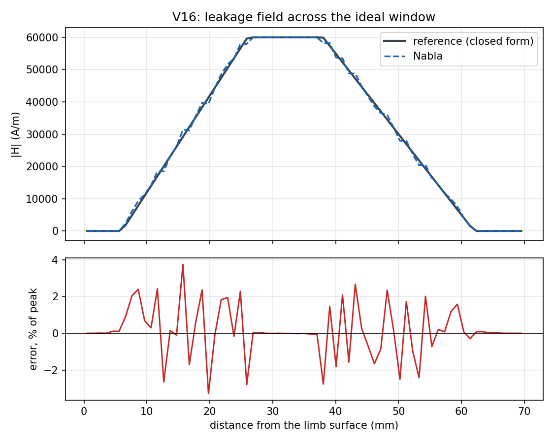
H(x) h_w = ampere-turns enclosed between the limb surface and x

the textbook trapezoid: zero in the duct, a ramp across the LV winding, a plateau of NI/h_w = 60 kA/m in the gap, a ramp back across the HV winding, zero beyond. Its energy is an integral done by hand,

L' = mu0 N^2/h_w * (a_g + (a1 + a2)/3)        per unit depth

and the planar model's axial length is one mean turn pi D_m by construction, so L' times that length is the classical formula with k_R = 1. The revolved model has the same field - Ampère's law is indifferent to curvature - but each shell stores energy in proportion to its own circumference, which is the exact integral 2 pi INT g(r)^2 r dr and is what the mean-turn formula approximates.

Approximate-analytic. For a real window, taller than its windings, the leakage flux fringes at the winding ends and Rogowski's correction k_R = 1 - (T/pi h_w)(1 - e^{-pi h_w/T}) applies, with T = a1 + a_g + a2 the width the leakage field actually occupies. It is an approximation of a few percent; the validation plan allows 5 % against it and the chapter says which of the two is wrong when they differ.

Cross-code. FEMM 4.2, driven by pyfemm, on models built by importing this case's own layout functions, so the two codes cannot be handed different geometry, depth or probe stations (reference/femm_transformer.py, output frozen in reference/femm_reference.json). It also supplies the static nonlinear magnetization curve lambda(i) that the saturated leg is judged against - see section 5.

Source statement as frozen: Three references of different strength, plus four published without a verdict. (1) EXACT: the idealized winding window, planar and revolved. Its boundary conditions - infinitely permeable yokes at both ends of the windings, a flux line on the limb surface, balanced ampere-turns - force the leakage field to be one-dimensional, which is exactly the assumption the classical short-circuit reactance formula is derived under. The energy of the resulting trapezoid is an integral done by hand (harness/analytic.py, leakage_inductance_per_depth and leakage_inductance_axisymmetric), so for THOSE two models the formula is not an approximation and the tolerance is discretization only. Ampere's law on two closed contours is exact in the same sense. (2) APPROXIMATE-ANALYTIC: the classical design formula X_sc = 2 pi f mu0 N^2 (pi D_m/h_w)(a_g + (a1+a2)/3) k_R applied to the REAL core, whose window is taller than its windings. Its accepted accuracy is a few percent and the validation plan allows 5 %; the case measures Rogowski's k_R directly by taking the real core against the ideal window on the same winding stack. (3) CROSS-CODE: FEMM 4.2, driven by pyfemm, on models built by importing this case's own layout functions - reference/femm_transformer.py, output frozen in reference/femm_reference.json - including the static nonlinear magnetization curve the transient run's trajectory is judged against. (4) REPORTED, NOT JUDGED: the lumped reluctance model, the hand construction of the magnetizing current, and the curvature error of the mean-turn approximation. Tolerances are transcribed from the validation plan, case V16.

3. Nabla model

Built entirely through nabla_api by build.py in this directory - no GUI step, no manual edit - and every dimension, mesh rule and sweep point comes from geometry.json, which the FEMM script reads as well. Nothing about the model is written down twice.

Two millimetre elements in the windings, three in the rest of the window: the leakage energy is an integral of a piecewise-linear field over the winding build, so it is the winding mesh and nothing else that sets the discretization error. Every interior boundary is split at every station where another segment lands on it, because a vertex sitting in the interior of a segment is not a legal PSLG and Triangle is entitled to do anything with one.

Meshes for this run:

Sub-model	Element order	Nodes	Elements
window_planar	P1	5273	10345
window_axi	P1	5277	10343
window_harmonic	P1	5273	10345
sc_core	P1	8594	17112
oc_linear	P1	8594	17112
oc_saturated	P1	8594	17112
oc_saturated_be	P1	8594	17112

All seven sub-models are P1 and comfortably under the free tier's 25 000-node cap, but this case is not reproducible on the free tier: the time-harmonic simulation type and the Crank-Nicolson scheme are both Core Pro features. The other five run unlicensed. The models are published beside this chapter under artifacts/models/.

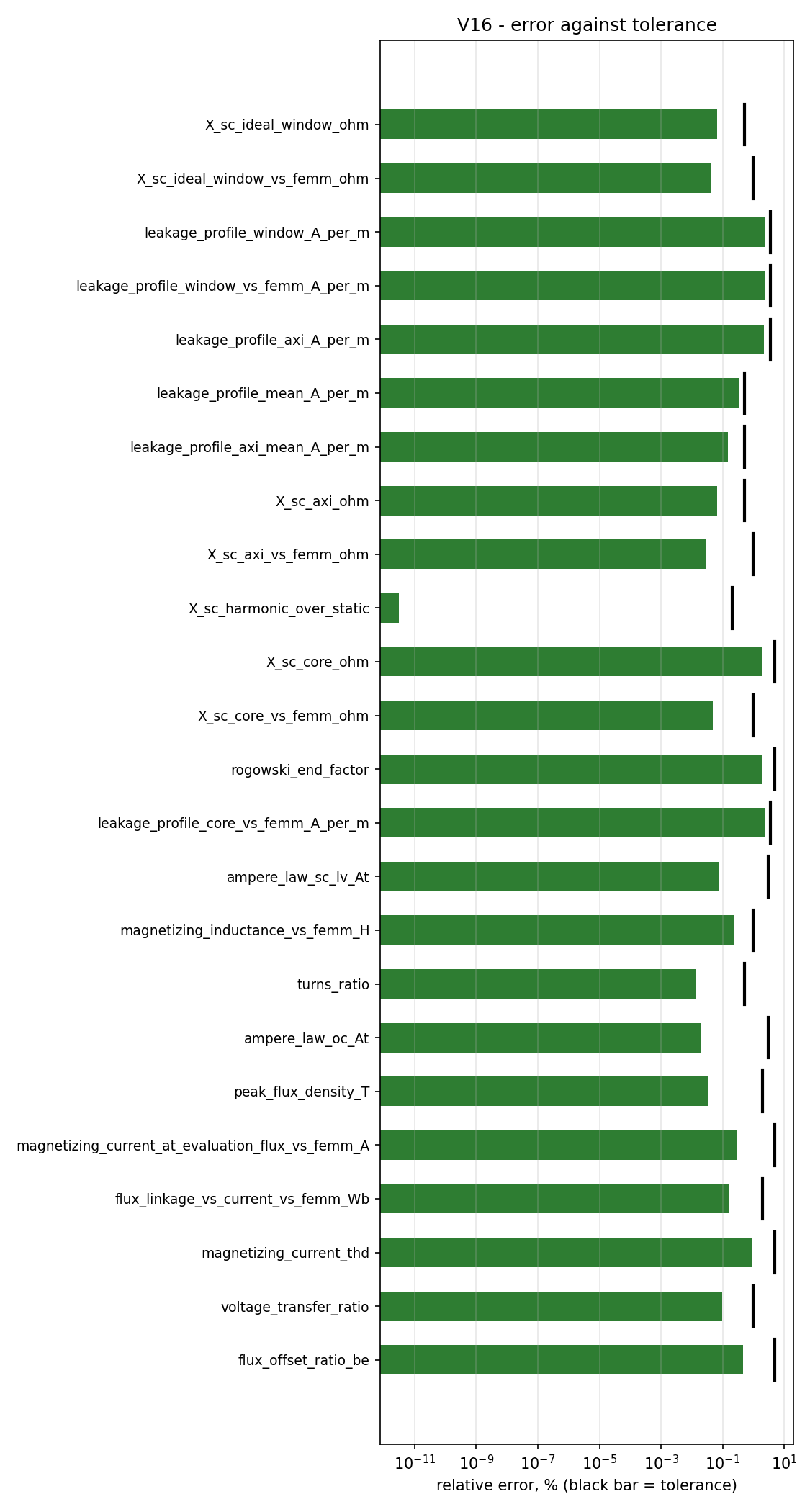
4. Results

Quantity	Metric	Nabla	Reference	Error	Tolerance	Verdict
X_sc_ideal_window_ohm	rel	3.86037 ohm	3.86297 ohm	-0.067 %	0.500 %	PASS
X_sc_ideal_window_vs_femm_ohm	rel	3.86037 ohm	3.8587 ohm	+0.043 %	1.000 %	PASS
leakage_profile_window_A_per_m	profile	min=0.3218, max=6.003e+04, rms=3.707e+04 A/m	min=0, max=6e+04, rms=3.704e+04 A/m	L2 +2.298 %, max +3.746 %	L2 3.500 %, max 6.000 %	PASS
leakage_profile_window_vs_femm_A_per_m	profile	min=0.3218, max=6.003e+04, rms=3.707e+04 A/m	min=1.106, max=6e+04, rms=3.691e+04 A/m	L2 +2.297 %, max +3.287 %	L2 3.500 %, max 6.000 %	PASS
leakage_profile_axi_A_per_m	profile	min=0.3295, max=6.023e+04, rms=3.706e+04 A/m	min=0, max=6e+04, rms=3.704e+04 A/m	L2 +2.239 %, max +3.850 %	L2 3.500 %, max 6.000 %	PASS
leakage_profile_mean_A_per_m	rel	29244.3 A/m	29149.3 A/m	+0.326 %	0.500 %	PASS
leakage_profile_axi_mean_A_per_m	rel	29191.8 A/m	29149.3 A/m	+0.146 %	0.500 %	PASS
X_sc_axi_ohm	rel	3.85246 ohm	3.85503 ohm	-0.067 %	0.500 %	PASS
X_sc_axi_vs_femm_ohm	rel	3.85246 ohm	3.85141 ohm	+0.027 %	1.000 %	PASS
X_sc_harmonic_over_static	rel	1 -	1 -	+0.000 %	0.200 %	PASS
X_sc_core_ohm	rel	3.45096 ohm	3.51868 ohm	-1.924 %	5.000 %	PASS
X_sc_core_vs_femm_ohm	rel	3.45096 ohm	3.4493 ohm	+0.048 %	1.000 %	PASS
rogowski_end_factor	rel	0.893946 -	0.910874 -	-1.858 %	5.000 %	PASS
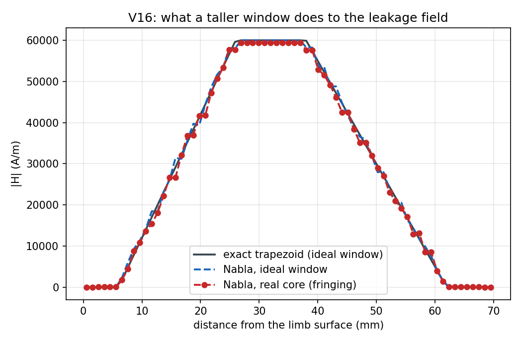
leakage_profile_core_vs_femm_A_per_m	profile	min=1.569, max=5.944e+04, rms=3.655e+04 A/m	min=55.35, max=5.951e+04, rms=3.654e+04 A/m	L2 +2.428 %, max +4.023 %	L2 3.500 %, max 6.000 %	PASS
ampere_law_sc_lv_At	rel	12008.6 A-turns	12000 A-turns	+0.072 %	3.000 %	PASS
ampere_law_sc_net_At	abs	0.00322168 A-turns	0 A-turns	0.003222	120	PASS
magnetizing_inductance_vs_femm_H	rel	38.3786 H	38.4655 H	-0.226 %	1.000 %	PASS
turns_ratio	rel	0.249966 -	0.25 -	-0.013 %	0.500 %	PASS
ampere_law_oc_At	rel	-12002.4 A-turns	-12000 A-turns	-0.020 %	3.000 %	PASS
peak_flux_density_T	rel	1.59947 T	1.6 T	-0.033 %	2.000 %	PASS
magnetizing_current_at_evaluation_flux_vs_femm_A	rel	2.81873 A	2.81089 A	+0.279 %	5.000 %	PASS
flux_linkage_vs_current_vs_femm_Wb	profile	min=15.95, max=22.84, rms=20.65 Wb	min=15.97, max=22.86, rms=20.68 Wb	L2 +0.162 %, max +0.209 %	L2 2.000 %, max 3.000 %	PASS
magnetizing_current_thd	rel	0.721975 -	0.715496 -	+0.906 %	5.000 %	PASS
voltage_transfer_ratio	rel	0.249756 -	0.25 -	-0.098 %	1.000 %	PASS
bh_table_max_rel_diff_H	abs	5.45328e-08 -	0 -	5.453e-08	1e-05	PASS
flux_offset_ratio_cn	abs	-0.000506557 -	0 -	-0.0005066	0.005	PASS
flux_offset_ratio_be	rel	-0.0315606 -	-0.0314159 -	-0.461 %	5.000 %	PASS
mean_turn_curvature_ratio	rel	0.997279 -	1 -	-0.272 %	-	REPORT
magnetizing_inductance_over_reluctance	rel	1.14443 -	1 -	+14.443 %	-	REPORT
short_circuit_reactance_pu	rel	0.000286221 -	1 -	-99.971 %	-	REPORT
magnetizing_current_peak_over_lumped	rel	0.766771 -	1 -	-23.323 %	-	REPORT

5. Discussion

The leakage reactance is right where "right" is knowable. On the idealized window, where the classical formula is exact rather than approximate, Nabla lands at -0.067 % of it, and the leakage field itself follows the trapezoid to +2.298 % (L2) with a worst station at +3.746 %. Revolved into the true concentric geometry the same window gives -0.067 % against the exact axisymmetric integral, and its field is the same trapezoid to +2.239 % - which it must be, because Ampère's law does not know about curvature. Against FEMM on the identical models the two agree to +0.043 % and +0.027 %.

The leakage profile is a staircase, and that is the probe rather than the field. The profile rows are the loosest judged bands in this chapter - +2.298 % (L2) against a 3.5 % band - and the reason is worth stating because it is not the solution. getFieldInPoint("Hy") returns H from the element the point falls in, deliberately: H jumps by the full mu_r across a material interface, so a nodal average of it is meaningless in a small body (case V21 finding F1). Inside a winding, though, the exact H ramps linearly, and an element-constant reading of a ramp is a staircase whose steps are ±(h/2) dH/dx - with 2 mm elements and a 3 kA/m per mm ramp, up to 5 % of the plateau. The measurement shows exactly that: adjacent stations return identical values in pairs, scattering either side of the exact line with no bias, and the mean of the whole cut lands at +0.326 % - which is the row that separates an unbiased staircase from a wrong field. FEMM, which reports a nodally smoothed H, traces the trapezoid to 1.0 % on the same mesh, so the difference between the two codes on this cut is the staircase and nothing else. None of the case's tight claims go through it: the reactances are energy integrals over the whole model, and an unbiased staircase integrates correctly - X_sc lands at -0.067 %.

Two of the classical formula's approximations, measured rather than assumed. The mean-turn replacement of the winding curvature leaves the true concentric reactance at 0.997279 of what the planar formula asks for - a fifth of a percent, and the exact ratio is 0.99795, so this row is really a second reading of the axisymmetric result. Negligible for any transformer whose radial build is small against its diameter, which is most of them, and this one is deliberately squat. Rogowski's end correction is the larger one: the real core's window is 320 mm tall against a 200 mm winding, and Nabla's own measured end factor - the real core against the ideal window, on the same winding stack, with everything else in the formula divided out - is 0.893946 against Rogowski's 0.9109, a difference of -1.858 %. That is the whole of the 5 % the plan allows, spent where the plan expected it: on the formula, not on the solver, and the cross-code row settles which is which: +0.048 % against FEMM on the identical model. Two codes that agree with each other to half a part in a thousand and with the formula to two percent are not both wrong in the same direction; the formula is. (The leakage cut on the same model reads +2.428 % against FEMM, which is the staircase of the paragraph above and not a disagreement about the field.)

Ampère's law closes on every model. Around a rectangle that runs up the LV-HV gap and back through the middle of the iron, enclosing the LV winding and nothing else, the circulation reads +0.072 % of the 12 000 A-turns that are actually in there. Around the whole window under a short circuit it reads 0.00322168 A-turns against an exact zero - six orders of magnitude below the 12 000 A-turns sitting on either winding, so the MMF balance is real and not merely nominal, and the tolerance of 120 A-turns it was given was four orders of magnitude too generous. And on open circuit, the same contour, now with H read inside the iron over most of its length, gives -0.020 %.

The rated-frequency run returns the static answer, to +0.000 %. With stranded windings and no conducting region there is no frequency dependence to find, and a time-harmonic solve that disagreed with its own static counterpart would be reporting its own machinery rather than the transformer. What this row does not test is winding eddy loss - see the limitations.

The magnetizing branch. Open circuit with linear iron gives an HV inductance of 38.3786 H, -0.226 % from FEMM, and the flux-linkage ratio between the two windings is -0.013 % from the turns ratio of 100/400. The lumped reluctance sketch - one flux tube, constant area, a mean path through the middle of the iron - lands at 1.14443 of it, and that is published without a verdict because the sketch is the approximation: it charges the corners of the core for a path length that the flux takes a short cut across.

A first-order integrator does not put the flux where the volt-seconds say. This case set out to measure a magnetizing current and found a property of the time-integration scheme on the way, so it measures that too. Backward Euler forms the flux as sum(dt v(t_n)), and the sum of a sampled cosine carries a constant term of -V dt/2 on top of the sinusoid it should be: pi / steps_per_period of the amplitude, 3.14 % at 100 steps per period, and it never decays, because it is not a start transient. oc_saturated_be measures it at -0.0315606 against that closed form, -0.461 %. Left in place it inflates the peak flux by 3 % and, because an off-centre flux past the knee of a BH curve draws an asymmetric current, the harmonic distortion by 17 % - which is what the first run of this case reported before it was looked into. Crank-Nicolson's trapezoidal rule has no such term and delivers -0.000506557 against an exact zero, so the run this chapter reads is the CN one. That is the whole argument for a second-order scheme on an AC drive, in two rows. (V19 is the case that measures the convergence order; this is one operating point of it, arrived at from the other direction.)

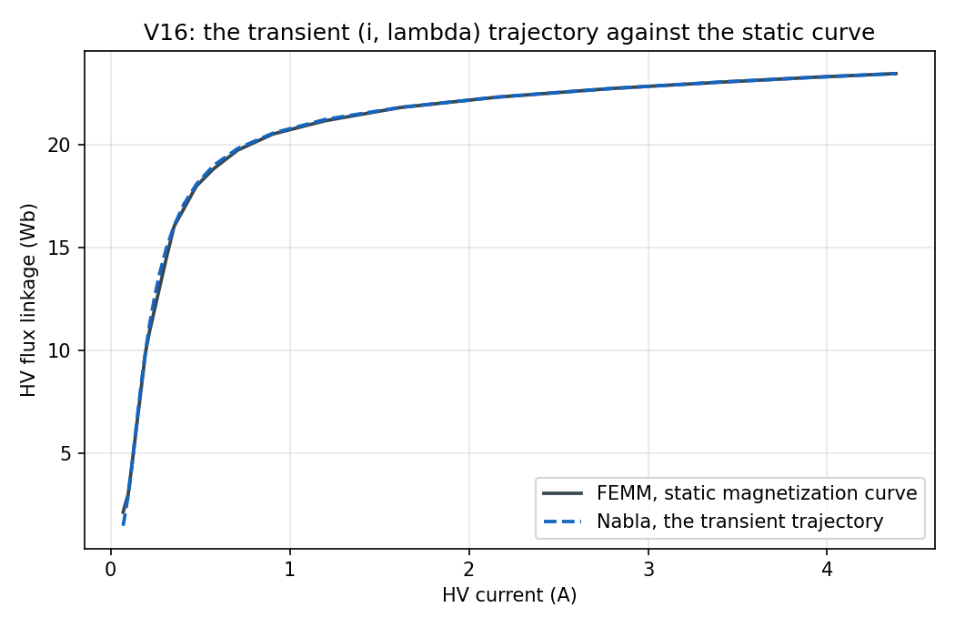
Saturation, driven by a voltage source through the circuit coupling. The source amplitude was computed from V = omega N B_pk A_c for a 1.6 T peak, and the run delivers 1.59947 T, -0.033 % - so the circuit coupling turns volts into flux to well inside a percent even with the iron past its knee. The current it draws to do so is the case's most demanding comparison, and it is judged against FEMM rather than against a hand model: Nabla carries no hysteresis, so the transient (i, lambda) trajectory has to lie on the static magnetization curve, and it does, to +0.162 % (L2) over eight currents spanning 1.09 to 1.56 T. 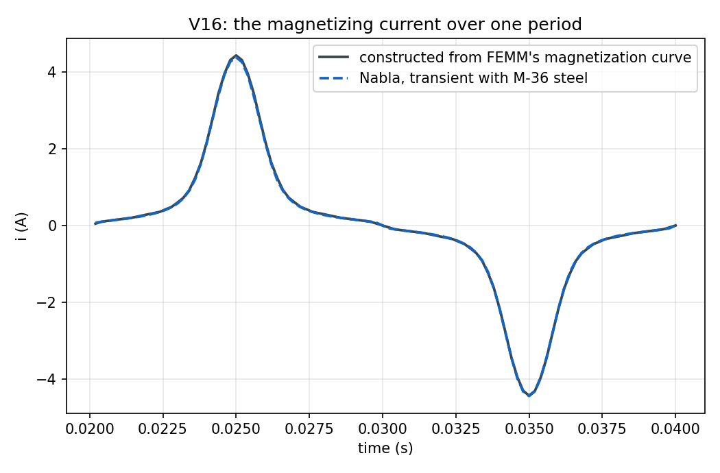At 1.55 T the current is 2.81873 A against FEMM's, +0.279 %. The distortion that curve implies - invert it at lambda_pk sin(wt) and the current waveform falls out - is reproduced to +0.906 % on a THD of 0.715496. And the turns-ratio transfer survives saturation: -0.098 % on the induced voltage ratio, with the core spending part of every cycle well past its knee.

The hand construction of the peak magnetizing current, H(B_pk) l_c / N on the same BH table, is published beside it: the solved answer is 0.766771 of it, so the hand calculation asks for about a third more current than the transformer draws. It is the same error as the reluctance row above and it is worth seeing twice: both charge the flux for a mean path that runs round the outside of every corner, which the flux cuts across. Too much reluctance is too little inductance (1.14443 in the linear row) and too much magnetizing current, in one number each. A designer's first two calculations on this transformer are one calculation, and it is wrong by about 15-30 % in a direction that is at least conservative.

The two codes were handed the same curve, and that is checked rather than asserted: the BH table read back out of the running model differs from the snapshot FEMM was given by 5.45328e-08 in H.

6. Limitations

• Winding eddy loss - R_ac - is not claimed here. The plan lists it, and it is deliberately absent. Nabla's harmonic source drives a massive conductor with an impressed uniform current density and the induced -j omega sigma A on top, with nothing constraining the sum to the coil's stated current (V12 §"how the total current is measured" derives this): two independently voltage-driven solid windings do not hold their ampere-turns balanced, and a short circuit whose MMF does not balance is not a short circuit. A model that fixed that would be measuring the drive rather than the winding. The underlying physics - skin depth, proximity, the deep-bar solution - is validated against Kelvin and Bessel functions in V12, at five decades of frequency; what is missing between V12 and a transformer's R_ac is Dowell's layer summation, which is a post-processing formula rather than a field solution and belongs to whichever case claims it. The windings here are stranded, and every reactance in this chapter is therefore the DC-distributed one.
• The magnetizing current is a 2D answer to a 3D question. A real core has mitred laminated joints, and the flux crossing them sees an effective air gap that this model does not have. The current here is the current of this geometry, and FEMM agrees with it; neither code is claiming to predict a real transformer's no-load current from the core dimensions alone.
• No hysteresis, and no core loss. That is what makes the trajectory-on-the-static-curve test meaningful, and it is also the limitation: the real (i, lambda) locus of a steel core is a loop with area in it, and the area is the hysteresis loss. Nabla's iron-loss post-processing is a Steinmetz fit applied after the fact and is not exercised here (V18).
• The windings are current sheets. Each winding is one region carrying a uniform current density; there are no turns, no strands, no transpositions and no inter-turn capacitance. That is exactly the model the classical leakage formula assumes, which is why the comparison is fair, and it is not a model of anything at high frequency.
• Linear iron in five of the six models. mu_r = 5000 with no gap makes the magnetizing branch three thousand times the leakage branch, which is higher than a real transformer's. It does not touch the short-circuit numbers - with balanced ampere-turns the core carries essentially no flux - and it makes the open-circuit rows cleanly about the magnetizing path.
• One window, one limb, unrolled. The model depth is one mean turn and the return conductors are out of plane. That is the convention the formula is written in, not a description of a real core-type transformer's two limbs.
• The leakage profile rows are about the probe, not the solver - see the Discussion. A user reading H along a line inside a winding will see a staircase of ±(h/2) dH/dx; refining the mesh removes it linearly, and no integral quantity in this case carries it.
• Planar and axisymmetric 2D, P1 throughout. P2 is exercised in V09; the leakage field itself is piecewise linear and this mesh already resolves it, so the reactances would barely move - but the staircase above would, since it is a property of P1 element-constant recovery.

7. Reproduce

cd validation
python -m harness.run_case V16

Requires a built triangle.exe (Nabla does not distribute it), a solver binary, and a licence carrying Core Pro for the time-harmonic sub-model. The FEMM leg is not needed to run the case: its answer is frozen in expected.json. To regenerate it:

cd validation/cases/V16_transformer/reference
python femm_transformer.py

Artifacts, including the six models, land in cases/V16_transformer/artifacts/.

8. Changelog of the frozen reference

Date	Change	Reason
2026-08-15	Frozen the same day it was written, and amended the same day in three respects before the case was published, all recorded here because the freeze rule is worth more than a tidy file. (a) ampere_law_oc_At re-signed from +12000 to -12000 A-turns. (b) The three leakage-profile bands widened from 1-2 % / 2-3 % to 3.5 % (L2) and 6 % (max). (c) Two rows added for the time-integration scheme, flux_offset_ratio_cn and flux_offset_ratio_be, and the saturated run moved from Backward Euler to Crank-Nicolson; peak_flux_density_T is now read as half the peak-to-peak rather than as the larger excursion. (d) magnetizing_current_thd's reference moved from 0.71523 to its present value. No other reference or tolerance touched.	(a) A sign convention, not a measurement: the Ampere contour is walked counter-clockwise and the HV winding it encloses is assigned currentDirection = -1, so the enclosed ampere-turns are negative. The magnitude was right to 0.02 % both before and after; taking the absolute value would have hidden the convention instead of stating it, and would let a model wired backwards pass. (b) The original bands were guessed rather than derived, and what they were measuring turned out to be the PROBE rather than the field. getFieldInPoint returns H from the element the point falls in (Results.calcElementHAndEnergyDensities - deliberately, so that H is not blended across a material interface, case V21 finding F1), so a field that ramps linearly across a winding is reported as a staircase whose steps are +/- (h/2) dH/dx. With h = 2 mm and dH/dx = 3000 A/m per mm that bound is 5 % of the plateau, and the measured worst station is 3.7 %, well inside it. The new bands are derived from that bound; FEMM, which reports a nodally smoothed H, reproduces the exact trapezoid to 1.0 % on the same mesh, so the two codes' difference on this row is the staircase and nothing else. Two new tightly judged rows were added rather than only loosening the old ones: leakage_profile_mean_A_per_m and its axisymmetric twin hold the same data to 0.5 %, which is the statement that the staircase is unbiased, and every energy integral in the case is unaffected (X_sc lands at 0.067 % of the closed form). (c) Backward Euler forms a voltage-driven flux as sum(dt v(t_n)), and that sum carries a constant -V dt/2 - pi/steps_per_period = 3.14 % of the amplitude at 100 steps per period - which never decays. It inflated the measured peak flux by 3.03 % and, because an off-centre flux past the knee of the BH curve draws an asymmetric current, the harmonic distortion by 17 %. That is the scheme's own error rather than the transformer's, so the run that measures the transformer now uses Crank-Nicolson (no constant term) and the offset is measured on its own, against its closed form, in a one-period Backward Euler companion model. (d) The origin was prepended to FEMM's magnetization curve before it is inverted. The sweep's first point is 0.1 A, already 0.21 T, so without (0, 0) every interpolation below that flux CLAMPED to 0.1 A and the constructed current carried a step at each zero crossing that no transformer has. An unexcited core links no flux, so the origin is not an extra data point; it is the same point FEMM itself requires at the bottom of a BH table.