V18 — Iron loss post-processing vs Steinmetz by hand

← Back to the validation dossier

Tier A (analytic) - priority P1 Reference frozen on 2026-08-15. Nabla 0.1.0, solver licence mode enforcing, run in 57.4 s.

This case shipped FAIL, found three defects, and now passes. As first built it measured Nabla's iron-loss post-processor returning 2.25x the Steinmetz hysteresis term and 1.985x the Steinmetz eddy term its own coefficients are defined for, plus a -2 % deficit along any iron/air boundary. All three factors were the same at every frequency and every flux density, two of them were predicted exactly by two lines of IronLoss.java that carried TODO comments asking about precisely these constants, and every scaling law in the model was correct to 1e-15 throughout - which is what made them constants to fix rather than a model to rewrite. They are fixed (case V18 findings F1-F3); the ratio rows below are now flat at 1, and the headline losses agree with the hand calculation to +0.402 %. Section 5 is written in both tenses: what was measured, and what the fix was.

1. Problem

One region, driven to a flux density that is uniform in space, sinusoidal in time, and known in closed form - and then asked what it lost.

The model is a plane-parallel cell, 60 x 40 mm, divided into four vertical layers with A = 0 on the two vertical walls and the natural condition on the two horizontal ones:

x:  0 ......... 20 ........... 40 ... 45 ......... 60 mm
    |   Iron    |    Bulk      | Coil |  Return    |
   A=0        (loss region is the first layer)    A=0

Nothing in it depends on y, so the problem is exactly one-dimensional and its solution is elementary (reference, section 1): B is constant in every current-free layer and proportional to the coil current. The drive current for each target B_peak is therefore solved for, not searched for.

Loss region	20 x 40 mm, 100 mm axial, 7650 kg/m³ - 0.612 kg
Coefficients	k_h = 0.02, alpha = 1.8, k_e = 5e-5 (W/kg, Hz, T)
Material	linear, mu_r = 1000, sigma = 0
Excitation	1000-turn coil layer, sinusoidal current, no circuit
Grid	50 / 200 / 400 Hz x 0.5 / 1.0 / 1.5 T - nine transient runs
Window	4 whole periods, 64 steps each: 257 field records
Formulation	Planar 2D, transient, P2 (6-node quadratic elements)
Controls	the same 50 Hz / 1 T cell with air around the iron, at 4 and 0.5 mm²

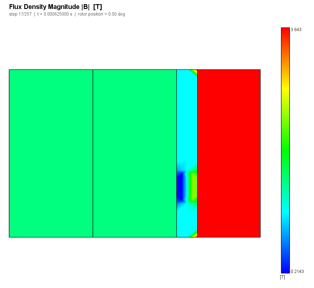
The picture is four flat bands, which is the point: B is constant inside each current-free layer and ramps across the coil. The other layers carry higher flux densities than the loss region - the Return layer sits at 2.43x it, because it encloses the full sheet current where the loss region encloses none - and at the 1.5 T point that is 3.6 T. Nothing in the case cares: the material is linear by declaration, there is no BH curve to saturate, and the only value any reference or any result uses is the one in the loss region.

Three modelling choices, and why each is not a convenience.

The exact solution is piecewise quadratic - linear in the passive layers, quadratic across the coil - so at P2 it lies inside the finite element space and the solved field is exact to round-off. The case does not assume this; it measures it. B_peak comes back with a profile error of +0.000 % and the probed waveform departs from B_peak |sin(2 pi f t)| by 2.96059e-15 x B_peak. That is what licenses a 1 % tolerance on a loss: no part of the gap below can be charged to the mesh.

Every layer of the nine cell models has the same mu_r. IronLoss used to read each element's |B| as the mean of its three nodal values, and a node on a material boundary carries a blend of the regions that touch it - 1 T of iron and 1 mT of air, here. With no permeability jump there is no blend, so the nine cell models measured the loss model rather than the nodal average, which is what let the two constants of 5.1 and 5.2 be measured without this on top of them. The two interface_* controls put the air back and measured what it cost (section 5.4) - which is how the third defect was found.

sigma = 0 in the iron. The Steinmetz eddy term is already a lumped model of the currents inside a lamination that a 2D model does not resolve. Letting the solver also induce a real eddy current in the same block would make B non-uniform and put a second, unrelated loss in the same region. The two are not meant to be summed, and this case does not sum them.

2. Reference

Derived in full in the case's reference notes; evaluated in harness/analytic.py, section Iron loss (V18). Nothing here is digitized or measured.

The field. d/dx((1/mu) dA/dx) = -J with A = 0 at both walls integrates once to B = mu (S - C) with S the enclosed sheet current and C = INT mu S dx / INT mu dx. Constant in every current-free layer, linear in the coil, exact.

The loss. P = m (k_h f B^alpha + k_e f^2 B^2). This is IronLoss.SteinmetzModel verbatim; it is what the steinmetzLoss API evaluates - checked here over the nine operating points, worst relative difference 0 - and it is the model whose three coefficients IronLossCoefficientsFitting solves for. With a known uniform B_peak, a known f and a rectangle's mass, it is arithmetic:

P(50 Hz, 1 T) = 0.612 * (0.02*50*1^1.8 + 5e-5*50^2*1^2) = 0.6885 W

The round trip. 42 noiseless (f, B, P) triples generated from the same three coefficients, written in the #Iron loss section format a material CSV uses, and handed back to fitIronLossCoefficients.

3. Nabla model

Eleven sub-models, built by build.py, one script and one parameter block. Each is meshed from scratch, solved as a linear transient with no saturation, no eddy currents and no circuit, and read with getResultsInRegion(region, "Iron AC Losses ...").

Sub-model	Element order	Nodes	Elements
cell_f050_b050	P2	803	380
cell_f050_b100	P2	803	380
cell_f050_b150	P2	803	380
cell_f200_b050	P2	803	380
cell_f200_b100	P2	803	380
cell_f200_b150	P2	803	380
cell_f400_b050	P2	803	380
cell_f400_b100	P2	803	380
cell_f400_b150	P2	803	380
interface_coarse	P2	2013	966
interface_fine	P2	15280	7539

4. Results

Quantity	Metric	Nabla	Reference	Error	Tolerance	Verdict
P_hyst_W	profile	min=0.1758, max=10.16, rms=4.261 W	min=0.1758, max=10.16, rms=4.261 W	L2 +0.000 %, max +0.000 %	L2 1.000 %, max 1.000 %	PASS
P_eddy_W	profile	min=0.01898, max=10.93, rms=4.132 W	min=0.01913, max=11.02, rms=4.164 W	L2 +0.773 %, max +0.773 %	L2 1.000 %, max 1.000 %	PASS
P_total_W	profile	min=0.1947, max=21.09, rms=8.332 W	min=0.1949, max=21.17, rms=8.364 W	L2 +0.385 %, max +0.402 %	L2 1.000 %, max 1.000 %	PASS
B_peak_T	profile	min=0.5, max=1.5, rms=1.08 T	min=0.5, max=1.5, rms=1.08 T	L2 +0.000 %, max +0.000 %	L2 0.100 %, max 0.100 %	PASS
B_waveform_max_dev	abs	2.96059e-15 -	0 -	2.961e-15	0.001	PASS
hyst_over_steinmetz	profile	min=1, max=1, rms=1 -	min=1, max=1, rms=1 -	L2 +0.000 %, max +0.000 %	L2 0.500 %, max 0.500 %	PASS
eddy_over_steinmetz	profile	min=0.9923, max=0.9923, rms=0.9923 -	min=0.9923, max=0.9923, rms=0.9923 -	L2 +0.000 %, max +0.000 %	L2 0.500 %, max 0.500 %	PASS
hyst_frequency_exponent	abs	1 -	1 -	-3.331e-16	0.02	PASS
hyst_flux_exponent	abs	1.8 -	1.8 -	-1.554e-15	0.02	PASS
eddy_frequency_exponent	abs	2 -	2 -	-2.22e-16	0.02	PASS
eddy_flux_exponent	abs	2 -	2 -	-8.882e-16	0.02	PASS
fit_Kh	rel	0.02 W/(kg Hz T^alpha)	0.02 W/(kg Hz T^alpha)	-0.000 %	0.500 %	PASS
fit_alpha	rel	1.8 -	1.8 -	-0.000 %	0.500 %	PASS
fit_Ke	rel	5e-05 W/(kg Hz^2 T^2)	5e-05 W/(kg Hz^2 T^2)	+0.000 %	0.500 %	PASS
steinmetz_api_max_rel_error	abs	0 -	0 -	0	1e-12	PASS
P_hyst_interface_coarse_W	rel	0.612 W	0.612 W	-0.000 %	-	REPORT
P_eddy_interface_coarse_W	rel	0.0759088 W	0.0759088 W	-0.000 %	-	REPORT
B_peak_interface_coarse_T	rel	1 T	1 T	-0.000 %	0.100 %	PASS
P_hyst_interface_fine_W	rel	0.612 W	0.612 W	-0.000 %	-	REPORT
P_eddy_interface_fine_W	rel	0.0759088 W	0.0759088 W	-0.000 %	-	REPORT
B_peak_interface_fine_T	rel	1 T	1 T	-0.000 %	0.100 %	PASS

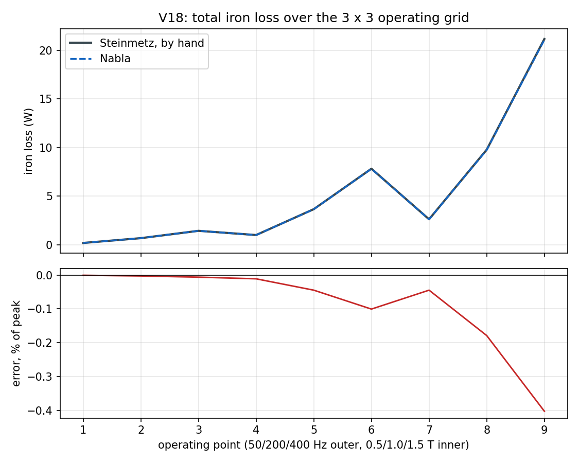
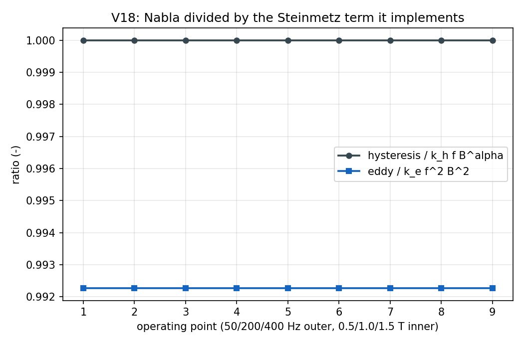
The second figure is the case in one picture: two flat lines. That they are flat is the load-bearing observation and it did not change with the fix - not a drift, not a spread, not something that grows with frequency or bends with saturation. What changed is where they sit: at 2.25 and 1.985 when the case was frozen, at 1 and 0.992 now.

5. Discussion

5.1 The hysteresis term counted each half period as a full cycle

Measured factor when the case was frozen: 2.25 at every point of the grid, matching the closed form 2 + 1/periods to 0.000 %. It is now 1, error +0.000 %, and P_hyst_W went from +125 % to +0.000 %.

IronLoss extracts turning points from the series of |B| and rainflow-counts them with the equivalent amplitude set to the cycle's full range (Bpk_eq = cycle.range). For B = B_peak sin(2 pi f t) that was wrong twice over, in ways that happen to compose:

• |B| has two humps per electrical period, each running 0 -> B_peak -> 0, and each was counted as a full cycle of range B_peak. One period was therefore charged 2 k_h B_peak^alpha where Steinmetz charges k_h B_peak^alpha. The amplitude was right - the range of |B| already is the signed amplitude, which is why hyst_flux_exponent came back as exactly alpha rather than bent - and the count was doubled. Working in |B| is not itself the mistake: it is the only defensible choice in 2D, where B rotates and has no fixed sign to rainflow. The mistake was that the weight was never adjusted for it. Fix: one closed excursion of |B| is emitted as half a cycle. Halving the amplitude instead would have given 2^(1-alpha) = 0.574x at alpha = 1.8 and would have bent the flux exponent with it.
• The three-point reduction leaves a residual stack, and rainflow() turned each residual into a full cycle at its raw range rather than closing it - its own TODO: decide if half cycle should be 0.5 or 1.0. Here that was worth exactly one more cycle per run, i.e. 1/periods of the answer, and worse, its size was not stable: the reduction's comparison is exact, so whether the residual collapsed depended on whether successive minima of |B| were bit-identical, and a real machine's |B| has no ties at all. This is why the case uses a short window: at four periods the term is 12.5 % and visible; at fifty it would have hidden inside the noise of a real model, still there and still wrong. It also made the machine summary the worst case, since MachinesPostprocessing.calcIronLoss takes one electrical period: 2 + 1/1 = 3. Fix: a post-processing window is always a whole number of electrical periods, i.e. a repeating history, so the turning points are rotated to begin at their global maximum before the reduction. The residual then closes on itself and carries no range, and the counted loss stops depending on the window length - asserted in IronLossSteinmetzTest.

5.2 The eddy term divided by pi^2 where 2 pi^2 is needed

Measured factor when the case was frozen: 1.98454, against the closed form 2 x (sampled <(d|B|/dt)^2> / exact) = 1.984545. It is now 0.992272, error +0.000 %, and P_eddy_W went from +98 % to +0.773 %.

calcEddyCurrentSpecificLossInElements formed (k_e / pi^2) <(d|B|/dt)^2>. For a sinusoid <(dB/dt)^2> = 2 pi^2 f^2 B^2, so k_e f^2 B^2 needs 2 pi^2 in that denominator - which is exactly what the method's own TODO: check the coefficient: 1 or 2 in the denominator (1 or 2 * pi^2) was asking. The answer, measured from outside on a problem whose value is known, is 2, and that is now the constant in the code.

The 0.77 % by which the measured factor sits below its target is sampling, not physics, and it survives the fix unchanged: the 4th-order stencil reads across the corner that |sin| has at every zero crossing and under-reads the slope there, while the rectangle sum over 257 records of a 256-step window over-counts by 1/256. The two partly cancel and the residue converges to zero as the sampling is refined - which is why the eddy row of IronLossSteinmetzTest is a 1 % statement where its hysteresis row is a 1e-9 one.

5.3 What survived the three constants: the law, and the fit

Everything else in the case was right before the fix and is unchanged after it, and that is not a small remark - a wrong constant is one line, a wrong law is a rewrite. It is also the reason the fix could be landed with confidence: none of the rows below were allowed to move.

• The fitted exponents are exact to round-off: hysteresis goes as f^1 and B^1.8 against f^1 B^1.8, eddy as f^2 and B^2 against f^2 B^2. The time step, the window normalisation, the element volumes, the mass and the B^alpha evaluation are all correct; a constant in front was all that separated the output from the model.
• The hysteresis/eddy split the validation plan asks for is clean. The two terms are separated by construction here (they scale differently in f and in B), and each is reported against its own reference rather than inferred from a total.
• The coefficient round trip is exact: k_h -0.000 %, alpha -0.000 %, k_e +0.000 % against the values that generated the data. So the fitting path and the evaluation path agree on what the model is; they disagree only about how many times to charge it.

5.4 The interface control

The two interface_* models are the same 50 Hz / 1 T cell with air around the iron, judged against the as-implemented value rather than against Steinmetz, because what they measure is the boundary and not the constants of 5.1 and 5.2.

As frozen, both read low and both roughly halved when the element size halved - -2.09 % / -2.26 % at 4 mm² and -0.76 % / -0.82 % at 0.5 mm², hysteresis and eddy, with the field in the interior of the iron still exact. That is the signature of the nodal blend: calcBabsInElementForIronLoss took the element's |B| as the mean of its three nodal values, those slots are averaged over every element sharing the node, and a node on the iron/air boundary therefore carried a blend of 1 T and 1 mT. Only the one element layer along the region's edge is affected, so the deficit scaled with the surface-to-volume ratio of the mesh rather than with anything physical - and the eddy term, quadratic in B, lost slightly more than the hysteresis term at B^1.8, exactly as it should.

It was a discretization artefact rather than a wiring constant, so a user could refine it away; but it was not small on a real machine, where a stator tooth is a few elements wide and bounded by air on three sides and 2 % on a 20 mm block is the optimistic end. The eggshell force and the region field energy already avoided the nodal slots for the same reason (Results.calcElementBFromA, which reads B = curl(A) off the element); the iron loss now calls the same helper, and both controls read

Mesh	Hysteresis	Eddy
4 mm²	-0.000 %	-0.000 %
0.5 mm²	-0.000 %	-0.000 %

with the interior field still exact (-0.000 %). The nine cell_* models did not move at all, which is the check that this changed the boundary layer and nothing else.

6. Limitations

Steinmetz is a fitted model for sinusoidal, unidirectional excitation. Its coefficients come from an Epstein frame or a ring sample under alternating flux (IEC 60404-2). This case supplies exactly that, which is what makes the hand calculation possible - and equally what makes it silent about a real machine, where the flux at a tooth root is elliptical, where the yoke sees minor loops riding on a fundamental, and where a PWM inverter adds harmonics the datasheet never saw. Nabla models no hysteresis: there is no B-H loop in the solver, the loss is a post-process on |B(t)|, and no part of it feeds back into the field. Rotational loss and excess (Bertotti) loss are not modelled at all. This paragraph is here so the machine chapters do not each have to write it.

What this case does not prove. That the loss of any machine is right - the grid here is one region at a known uniform flux density, which no machine part is. That the rainflow minor-loop extraction is right for a waveform with genuine minor loops: a rectified sine has none, so this case pins the counting convention and says nothing about the reduction on a complicated waveform. That the alpha recovered from a real datasheet is meaningful - only that the fit recovers what generated it.

What the three factors meant for the register, and what changed. Any iron loss quoted anywhere else in this dossier or by the GUI is computed by the code measured here. Before 2026-08-15 it was about 2.2x the Steinmetz model whose coefficients the material library ships - and about 3x on the machine summary, the PDF report's loss table, the loss-breakdown pie and the anchors behind every efficiency and loss curve, because those take a one-period window and so carried the whole of the residual term. An iron loss from Nabla had to be read as an indicator rather than a watt figure, and this chapter was the reason a reader knew that.

The three defects are now fixed (case V18 findings F1-F3) and the ratio rows are flat at 1, so an iron loss from Nabla is a watt figure, within the model's own limitations above. Two things follow for a reader of anything older: every iron loss printed by a build from before that date was high by those factors, and the ratios built from two anchors were not - PerformanceAnalysis.fitFluxExponent divides one iron loss by another, so a common constant cancelled there and those curves keep their shape. This case is the regression test that holds the fix in place, together with IronLossSteinmetzTest, which drives the same chain on a synthetic |sin| series in under a second and did not exist before: no Java test anywhere touched IronLoss, which is how two constants sat behind TODO comments through several releases.

7. Reproduce

cd validation
python -m harness.run_case V18

Eleven sub-models, about a minute in total; the case is in the fast nightly tier. --keep-work keeps every mesh and solution. The generated specific-loss table the round trip is fitted from is published as artifacts/synthetic_loss_table.csv, and every solved model as artifacts/models/*.nbl.

Date	Change	Reason
2026-08-15	The six AS-IMPLEMENTED rows were re-frozen: hyst_over_steinmetz 2.25 -> 1.0; eddy_over_steinmetz 1.9845447254157118 -> 0.9922723627078559; the four interface controls halved with them (1.377 -> 0.612 W and 0.15181767149430198 -> 0.07590883574715097 W).	These six are the case's AS-IMPLEMENTED rows - they describe what the post-processor evaluates, not what physics says - and case V18 findings F1, F2 and F3 changed what it evaluates. F1: IronLoss.rainflow now weights each closed excursion of