V20 — Solver-option invariance matrix

← Back to the validation dossier

Tier S (solver-internal) - priority P1 Reference frozen on 2026-08-15. Nabla 0.1.0, solver licence mode enforcing, run in 203.2 s.

1. What this chapter claims

Not a physics result. Nabla offers a user half a dozen switches that are supposed to be choices of method - which linear solver, which time-integration scheme, which element order, which sliding band, how many axial slices, monolithic or staggered field-circuit coupling - and this chapter asks the only question those switches owe an answer to: does moving one of them move the answer?

Two models, fifteen solves. Each model is solved once as a baseline and once per option, with exactly one thing moved, and every difference is compared against zero.

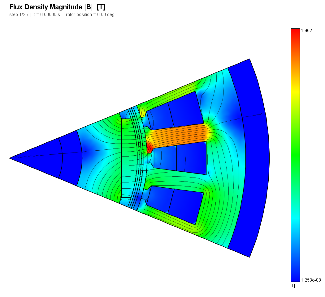
m_*	a 24-slot / 8-pole surface-PM machine from Nabla's parametric PMSM module: motion, an averaging sliding band, saturating M-19 steel, one electrical period at 24 rotor positions, 7564 nodes
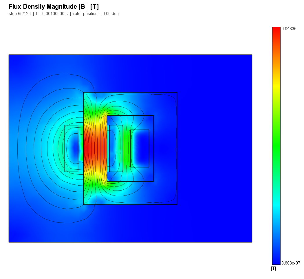
e_*	a 200-turn coil on a linear core with a copper plate in the window, fed from a 100 V step through 20 ohm: eddy currents, a circuit whose coil current is an unknown, 128 steps over 2 ms, 2035 nodes
Options	SimplicialLDLT / Conjugate Gradient - Backward Euler / Crank-Nicolson - P1 / P2 - averaging band / legacy stitch band - 1 / 4 skew slices - monolithic / staggered coupling

2. Which rows are judged, and why the rest are not

An invariance is only claimable where the two runs being differenced solve the same problem. Three bands, all frozen before the case was pointed at Nabla:

Band	Value	What the two runs share
identity	1e-5	the same algebraic system; only the iteration stopping point can separate them (the machine's Newton loop stops at 1e-6)
linear solver	5e-4	the plan's 0.05 % for Conjugate Gradient against the direct factorization

A third band was frozen with the case - coupling, 5e-3, the plan's 0.5 % for monolithic against staggered field-circuit coupling - and it no longer judges anything. It assumed the two couplings differ only by a one-step O(dt) lag; §4.1 is the measurement that refuted that, and staggered coupling with eddy currents on is now a combination the solver warns about. A row cannot be judged against a configuration Nabla declares unsupported, so it is reported. The supported limit is still measured, by the same two couplings with the eddy term switched off.

and everything else is published without a verdict, because differencing two discretizations measures the mesh and not the option surface. P1 against P2 is a different discretization on a mesh that has to be regenerated; the legacy stitch band is a different geometry as well, since it places the two airgap surfaces at another pair of radii. Their numbers are in §5, and they are the right thing to read the judged bands against.

The one identity that needed care is skew. Nabla folds an N-slice run back to a single slice whenever the skew angle is zero, so a literal 0 degrees never reaches the multi-slice code path. The case therefore asks for 4 slices at 1e-6 degrees - slice offsets of ~2e-8 rad, i.e. four copies of the same problem solved jointly - which exercises the whole multi-slice machinery with the physics it normally introduces switched off.

3. What passes, and it is most of it

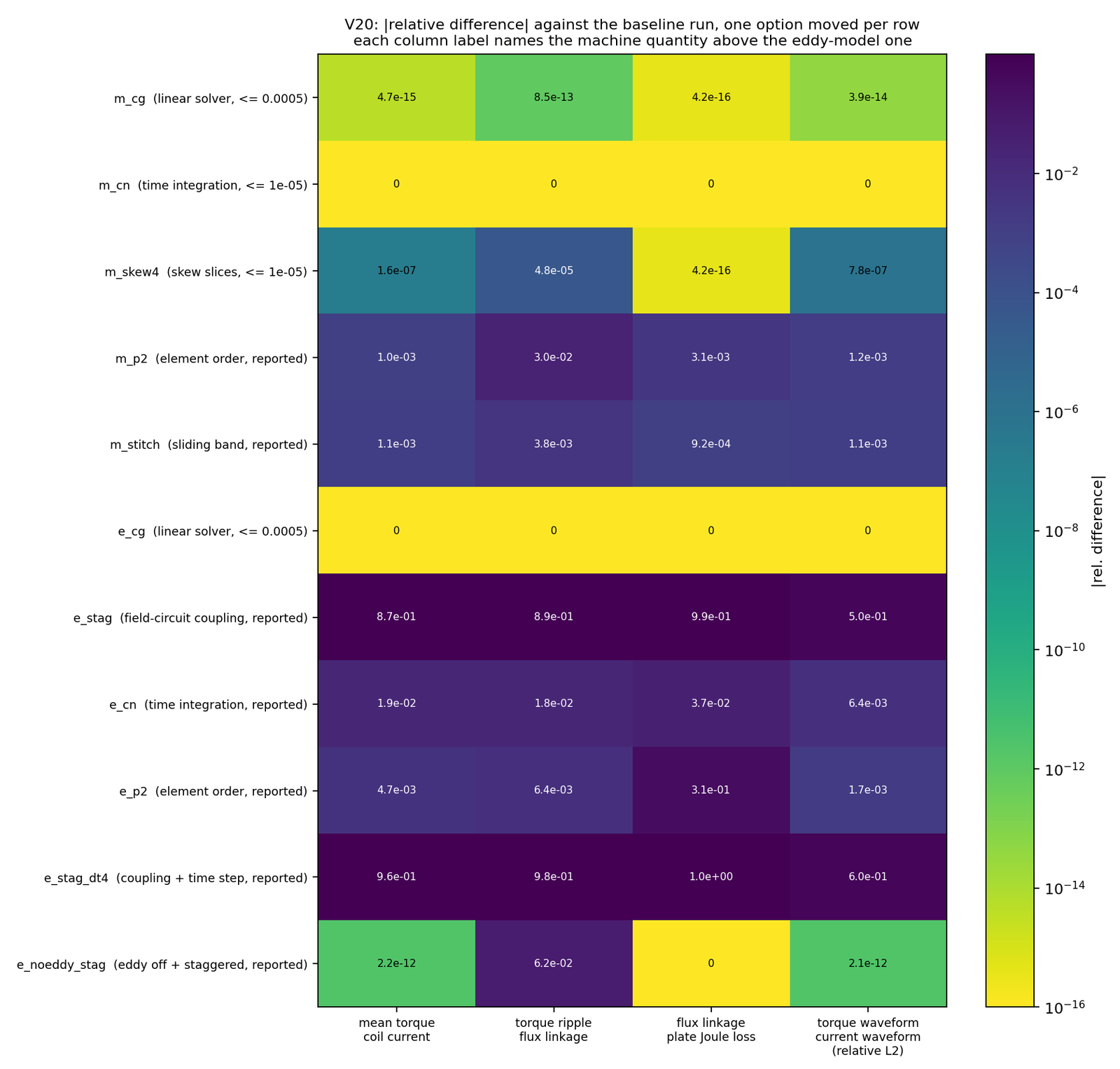
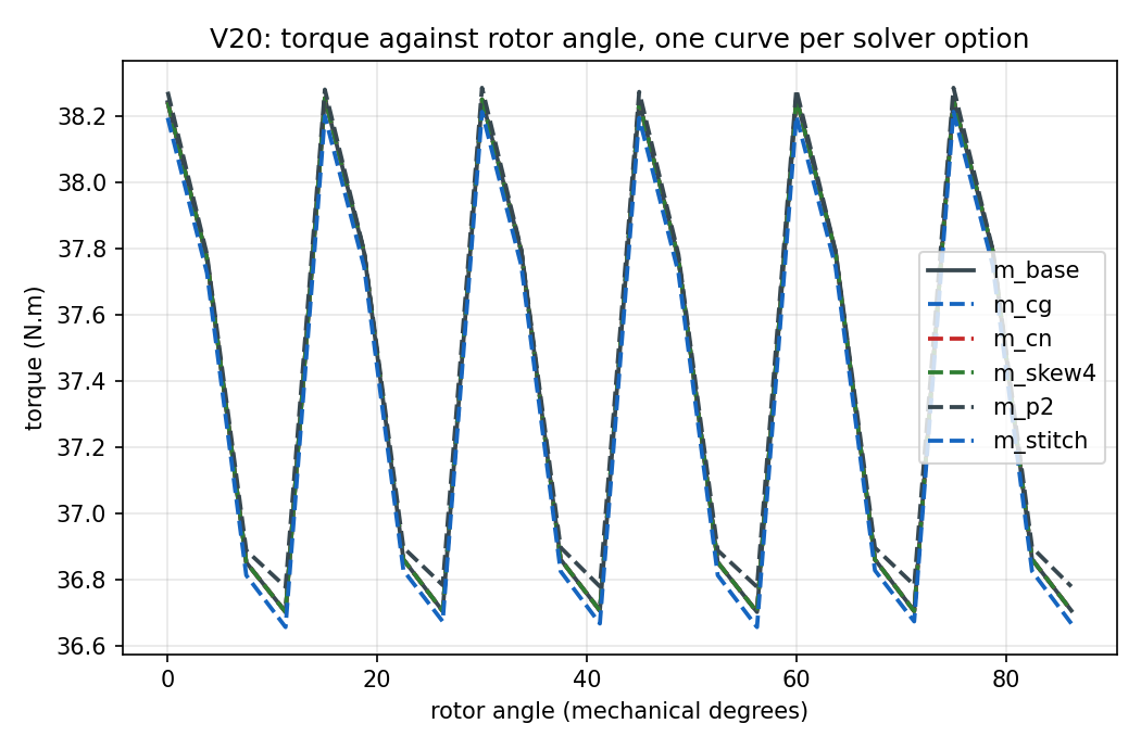
Conjugate Gradient is bit-identical to the direct factorization, on both models. Mean torque, peak flux linkage and the whole 24-point torque waveform of the saturating machine all differ by exactly 0, and so do the eddy model's coil current, flux linkage, plate Joule loss and 128-point current waveform. That is a stronger result than the 0.05 % the plan asks for, and it is stronger than it looks: the machine is nonlinear on purpose, so the iterative solve is running inside a Newton loop, where an inexact solve gets to feed back on itself. CG is asked for a 1e-12 residual, so the row measures agreement and not CG's stop rule.

Backward Euler and Crank-Nicolson are bit-identical on the machine, also exactly 0 on every quantity - which is what they owe: nothing in that model has a time derivative, so theta multiplies only terms that are zero and the two schemes are the same matrix. The eddy model, which does have one, separates them by 0.0187491 on the knee current; that is a real truncation error and V19 is the chapter that judges it.

The monolithic and staggered couplings agree to 2e-12 with eddy currents off - see §4, where that number is the diagnosis rather than the result.

4. Two findings, and what came of them

4.1 The staggered field-circuit fallback leaves the physics when eddy currents are on

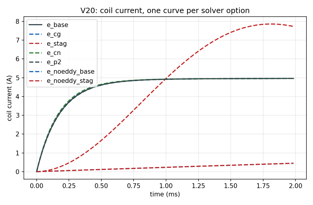
NABLA_MONOLITHIC=0 is the documented A/B switch back to the legacy staggered coupling. On this model it does not miss a tolerance - it misses the source:

	monolithic (default)	staggered (NABLA_MONOLITHIC=0)
coil current at 2 ms, as a fraction of V/R	0.99207	1.54585
knee current, relative to monolithic	-	-0.872859
plate Joule loss, relative to monolithic	-	-0.990504

A series RL loop fed from 100 V through 20 ohm cannot carry more than V/R = 5 A in any steady state, under any time step and any discretization: the source has no other energy to give and the inductor stores none once di/dt is zero. The window is about ten circuit time constants. The default settles at 0.99207 of that bound, as it must. The staggered path ends at 1.54585 of it, having crossed V/R and kept going.

The pre-registered explanation for a monolithic/staggered difference is a one-step lag, which is O(dt). The case refutes its own explanation: run the same pair at four times the time step and the difference grows by 1.09843, where a lag owes 4.

So the same two couplings were run once more with the sigma dA/dt term switched off - the one thing that distinguishes this model from the circuit-only case the staggered path was written for. With eddy currents off they agree to 2.15593e-12 on the coil current and 2.09056e-12 on the whole waveform, and the flux linkage carries exactly the one-step lag the theory predicts (-0.0621553). The staggered coupling is not broken; the combination of the staggered coupling with the eddy-current reaction is. That is the combination the monolithic path was built to replace, and this chapter is the measurement of what it replaced.

The mechanism, read out of the staggered branch: calcCircuitCoilsExtEMF hands the circuit an explicit, one-step-lagged EMF correction while the MNA represents the coil as a pure inductance L/dt, and L comes from the adjoint on the eddy-augmented Jacobian, so it is itself a function of dt. An eddy-shielded coil is a lossy, frequency-dependent impedance; no single L makes the circuit side right, and refining dt renews the model error rather than reducing it - which is precisely why the ratio above is 1 and not 4. This is a structural limit of the split, not a wiring defect: the monolithic path does not repair it, it avoids it by making the coil current a field unknown.

What shipped: the solver now prints a warning when NABLA_MONOLITHIC=0 suppresses a coupling that would have been monolithic and eddy currents are enabled, naming the mechanism and the bound it violates. NABLA_MONOLITHIC=0 is a debugging switch, not a supported alternative, and this chapter's e_stag rows are therefore reported rather than judged - they remain in the register as the regression that would notice if the default path ever picked up the same behaviour. Details in case V20 finding F1.

4.2 The skew identity was measuring the sliding band

The degenerate-limit identity failed on the case's first run - mean torque off by 3.26e-5 and the torque waveform by 1.33e-4, against a 1e-5 band - and the diagnosis turned out to have nothing to do with skew.

The single-slice baseline disagrees with itself by the same amount. This machine is exactly antiperiodic over half an electrical period, so λ[k+12] must be −λ[k] and T[k+12] must be T[k]. At Nabla's default band subdivision the baseline violates its own antiperiodicity by 4.6e-4, and the four-slice run violates its own by the same order at the complementary rotor positions. Wherever a run is self-consistent the two runs agree to 1e-14. There was no skew defect to find: the slices merely resample a position-dependent error the baseline already had.

That error is the band's. buildSlidingBandConstraints couples a moving node to its two bracketing stationary ring nodes by linear interpolation, so the band carries an O(h²) error in the ring pitch that depends on where the rotor angle falls relative to it. Refining the mesh cannot reach it - the machine PSLG meshes with -Y, so the ring nodes are the air-surface subdivision points and a mesh_max_area leaves them alone (3.2k to 12k nodes moved the violation 4.56e-4 to 5.85e-4, i.e. not at all). Refining the ring reaches it, at clean second order:

ring nodes	self-antiperiodicity	four slices against one, waveform L2
53 (Nabla's default here)	4.56e-4	1.33e-4
200	3.45e-5	1.02e-5
800	1.71e-6	7.76e-7

Two things this rules out, both measured: it is not the nonlinear solve - the difference is identical to four digits at nonlinear tolerances of 1e-6, 1e-10 and 1e-13, so it is neither round-off nor a Newton stopping point - and the flux linkage is not unaffected; its waveform moves by 1.8e-4, larger than the torque's. The first run's reading of exactly 0.0 there was a scalar peak seen through a 32-bit float (below).

What shipped: the case now pins the band to 800 ring nodes, so its own reproducibility justifies the identity band it was already frozen at. The tolerance was not widened. The half-period antiperiodicity check is the better instrument for this class of error and needs no A/B at all - one run answers it. Details in case V20 finding F2.

Found while chasing it, and now fixed: MachineUtilsAPI.buildPhaseSeriesResult narrowed every machine time series to a 32-bit float on its way to the Python API (series.get(i).floatValue()), in the middle of a double-to-double copy, so torque, flux linkage, back-EMF and phase current all reached a scripted user with about seven significant digits. It was three orders of magnitude too small to explain either finding, but it did distort the evidence for 4.2 by rounding a real difference to exactly zero. Every number in 4.2 was measured with it removed.

5. What the case measures about itself

The discretization differences, published with no verdict, and the reason the judged bands mean anything:

	machine	eddy
P2 against P1, primary quantity	0.000997323	-0.00470316
P2 against P1, waveform L2	0.0012005	-
P2 against P1, Joule loss	-	0.307841
stitch band against averaging band	-0.00110122	-

Element order moves this machine's torque by 0.000997323 and the eddy model's plate loss by 0.307841 - the second is large because a Joule loss is what an under-resolved skin depth gets wrong first, and it is the honest statement of what the eddy leg's own mesh is worth. Both are far above every judged band, which is the point: the options this chapter judges are invisible next to the mesh, and that is the result.

And what the options cost, which is the other half of an option matrix:

option	wall-time ratio against its baseline
4 skew slices	2.56256
P2, machine	5.38686
P2, eddy	7.08896

6. Limits

• Two models, not a survey. Planar 2-D throughout; no axisymmetric run, no time-harmonic run, no thermal run. An option that is only wrong in axisymmetry would pass this chapter.
• One mesh per model. An invariance is a comparison of two runs on the same mesh, so nothing here says anything about mesh convergence; V09 does that.
• The band comparison is a control, not a claim. The two sliding bands are built into different machines, so §5's stitch-band row is a difference between two models and cannot be tightened into an invariance. V05 carries the same control for the same reason.
• The coupling row is model-dependent. 4.1 is measured on one eddy-current model at one time step. What generalises is the mechanism and the V/R bound, not the 87 %.