V23 — Loss to thermal handoff on a machine

← Back to the validation dossier

Tier A+S (analytic + self-consistent) — priority P2 Reference frozen on 2026-08-16. Nabla 0.1.0, solver licence mode enforcing, run in 52.5 s.

This chapter shipped FAIL, found two defects, and now passes. Every physics row passed on the first run, most of them three orders of magnitude inside their tolerance. What failed was a self-consistency check between two rows of Nabla's own machine summary — the Joule loss and the phase resistance disagreed by a factor of exactly 2.000 — and the failing row was added after that run, by this case, because reading the two numbers next to each other is what found it. Both that defect and the silent iron-loss zeroing beside it were fixed in Nabla on 2026-08-16; the summary now reports 1059.25 mOhm against the loss-implied 1.05925 Ohm, and the row that failed reads its reference to +0.000 %. The findings are kept in §6 as found, in the past tense, because a finding that is deleted when it is fixed cannot regress. See case V23 findings F1 and F2.

1. Problem

Nabla has an electromagnetic post-processor that reports a machine's losses per part, and a thermal solver that takes volumetric heat sources per region. This case is the first thing in the register that connects the two, on one machine, in one script, and checks that the watts survive the journey.

Sub-model	Physics	What it does
em	magnetostatic rotor sweep, P1, averaging sliding band	the V05 surface-PM machine, loaded at Id = 0, Iq = 30 A peak, 1500 rpm, one electrical period at 72 steps. Produces three numbers: winding Joule loss, stator iron loss, rotor iron loss.
stack_p1	steady conduction, planar, P1	those three numbers as volumetric sources in a nine-layer concentric-annulus model of the same radial stack, cooled by a film on the frame
stack_p2	the same at P2	the same problem, quadratic elements

The machine is V05's, read and not copied. build.py loads ../V05_spm_pmsm/design.json and publishes its SHA-256 (c66beba308cac8fd5e87ef113a1008f4648d53dd8fcc3ea30f2b62029981c158), so the two chapters provably describe one motor and a change to V05's machine cannot walk away from V23's stack unnoticed. Everything V23 adds is in thermal_stack.json: one radius, nine conductivities, a film coefficient, and where each loss is deposited.

1.1 The thermal model, stated rather than discovered

It is a 1-D radial idealization, and every one of these is a modelling statement a reader is entitled to disagree with:

#	Layer	r (mm)	k [W/(m K)]	Source
1	Shaft	13.5 → 18.5	45	—
2	Rotor Core	18.5 → 28.5	25	rotor iron loss
3	Magnets	28.5 → 32.5	9	—
4	Rotor Sleeve	32.5 → 33.0	15	—
5	Air Gap	33.0 → 34.0	0.030	—
6	Stator Sleeve	34.0 → 35.0	0.20	—
7	Slot And Teeth	35.0 → 50.0	14.2149 (computed)	winding Joule loss
8	Stator Yoke	50.0 → 60.0	25	stator iron loss
9	Housing	60.0 → 66.0	167	—

• Radii 1–8 are V05's own derived stack. Two of them are not really radii in V05 — the flat-bottom magnet's inner face is a chord and the rectangular slot's bottom is a straight line — and treating them as radii is the first idealization. The frame's outside is this case's own addition, put at V05's outer-air radius, which makes it 6 mm thick by coincidence rather than by choice.
• The toothed layer is homogenized, and its conductivity is derived: at the mid-slot radius the teeth occupy 0.550621 of the circumference (24 slots of 5 mm out of 2 pi x 42.5 mm), so k = f k_tooth + (1-f) k_slot with 25 and 1.0 W/(m K). The copper loss is spread uniformly over that whole layer, teeth included.
• The shaft bore is adiabatic, and it gets that way by carrying no boundary condition at all — an unmarked thermal boundary is natural Neumann. Marker 1 is reserved as "no BC", so nothing is inherited there.
• The airgap conducts and does not convect. k = 0.030 is still air. A rotating gap does better than that (Taylor–Couette), so the rotor here runs hotter than it would.
• The frame's film coefficient is fitted. h = 120 W/(m^2 K) at 40 °C ambient — a totally-enclosed fan-cooled frame of this size with its fin area lumped in, and, since a 2-D cross-section has no end surfaces at all, every axial path out of the machine lumped in with it. The validation plan V23 requires this to be said out loud. It is said again in §7, because it is the single reason this chapter is a demonstration of the chain and not a thermal prediction of this machine.

2. Reference

The thermal leg is a closed form. Nine concentric annuli, each homogeneous, each with its own uniform source: inside layer i the steady radial equation (1/r) d/dr(r k dT/dr) + q = 0 has the general solution

T_i(r) = -q_i r² / (4 k_i)  +  A_i ln r  +  B_i

so the exact answer is a 2N-unknown linear system — one bore condition, two per interface, one film condition. That is harness.analytic.layered_cylinder_*, tested on its own in validation/tests/test_analytic_thermal_stack.py (degenerate limits, the governing equation in integral form at a station inside every layer, and the invariances). Standard statements of the two- and three-layer cases: Carslaw & Jaeger §7.2; Incropera §3.3 and §3.5.

The handoff leg is conservation, which needs no closed form at all: what the magnetic post-processor reported, what the thermal solution carries across a contour in the frame, and what the film removes are the same power.

One thing is frozen and one thing is not, and the distinction is the case. The exact solution is a function of the heat put into it, and what is put into it is what Nabla's own loss post-processor reported. So expected.json freezes the tolerances — before the run, as the validation plan §3.3 requires — and reference() re-solves the closed form each run on that run's losses. Freezing a temperature would freeze a number that is right for exactly one loss figure, and the first time the loss post-processor changed, the case would quietly become a comparison against a machine that no longer exists.

The loss figures themselves are therefore judged against nothing and published as report rows. That is the honest verdict for them: there is no independent reference for the losses of a machine that was never built, and a textbook loss density would be a tolerance chosen to be met.

3. Nabla model

Sub-model	Element order	Nodes	Elements
em	P1	3122	6009
stack_p1	P1	41021	81423
stack_p2	P2	163465	81423

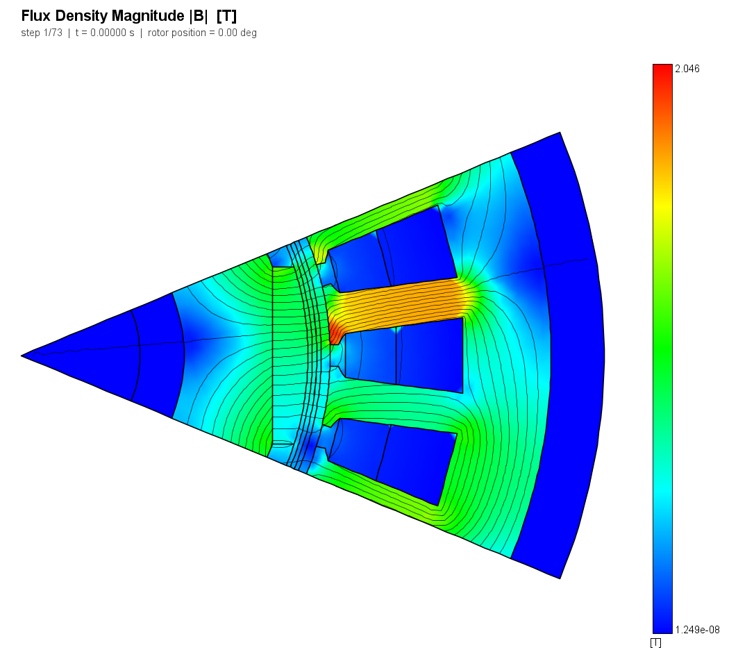
The electromagnetic run differs from V05's in three deliberate ways, all of them because V23 asks a different question:

• the back-EMF stage is off — every number this case takes out of the machine is a loaded one, and the no-load sweep would double the run for nothing;
• 72 steps per period instead of 180 — the losses are a period average and a rainflow count of |B| over one period, both converged long before V05's cogging waveform is;
• end-winding resistance is ON, where V05 turned it off. V05 compares two field solutions and an analytical add-on is in neither. This case asks what the winding dissipates, and the end turns of a 100 mm stack dissipate a real share of it. Where that heat then goes is the thermal model's idealization: a 2-D cross-section has nowhere to put an end winding, so it enters the slot layer with the rest.

The iron-loss coefficients are not re-fitted to the assigned material, and that is finding F1 — see §6.

4. Results

Quantity	Metric	Nabla	Reference	Error	Tolerance	Verdict
loss_copper_W	report	1429.99 W	- W	-	-	REPORT
loss_stator_iron_W	report	5.83927 W	- W	-	-	REPORT
loss_rotor_iron_W	report	0.00218232 W	- W	-	-	REPORT
loss_total_W	report	1435.83 W	- W	-	-	REPORT
loss_sum_minus_total_W	abs	0 W	0 W	0	0.05	PASS
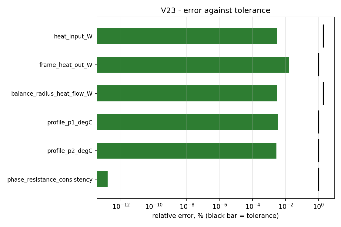
heat_input_W	rel	1435.88 W	1435.83 W	+0.003 %	2.000 %	PASS
frame_heat_out_W	rel	1436.07 W	1435.83 W	+0.017 %	1.000 %	PASS
balance_radius_heat_flow_W	rel	1435.88 W	1435.83 W	+0.003 %	2.000 %	PASS
winding_temp_p1_degC	abs	365.023 degC	365.027 degC	-0.00431	0.8	PASS
winding_temp_p2_degC	abs	365.03 degC	365.027 degC	0.003213	0.5	PASS
rotor_surface_temp_p2_degC	abs	371.674 degC	371.659 degC	0.01421	0.5	PASS
magnet_temp_p2_degC	abs	371.674 degC	371.659 degC	0.01421	0.5	PASS
housing_surface_temp_p2_degC	abs	328.582 degC	328.576 degC	0.006131	0.5	PASS
airgap_drop_p2_K	abs	6.64328 K	6.63228 K	0.011	0.8	PASS
profile_p1_degC	profile	min=328.6, max=371.7, rms=358.3 degC	min=328.6, max=371.7, rms=358.3 degC	L2 +0.003 %, max +0.005 %	L2 1.000 %, max 2.000 %	PASS
profile_p2_degC	profile	min=328.6, max=371.7, rms=358.3 degC	min=328.6, max=371.7, rms=358.3 degC	L2 +0.003 %, max +0.004 %	L2 1.000 %, max 2.000 %	PASS
winding_p1_minus_p2_K	abs	-0.00752342 K	0 K	-0.007523	0.8	PASS
profile_p1_minus_p2_max_K	abs	0.00963499 K	0 K	0.009635	1.5	PASS
phase_resistance_consistency	rel	1 -	1 -	+0.000 %	1.000 %	PASS
phase_resistance_implied_ohm	report	1.05925 ohm	- ohm	-	-	REPORT
continuous_current_estimate_A	report	17.7837 A	- A	-	-	REPORT
winding_hotspot_margin_K	report	-210.03 K	- K	-	-	REPORT
iron_split_sensitivity_K	report	0.111725 K	- K	-	-	REPORT
current_density_A_per_mm2	report	9.44978	-	-	-	REPORT
efficiency_percent	report	80.3647	-	-	-	REPORT
mech_power_kW	report	5.87665	-	-	-	REPORT
phase_resistance_mohm	report	1059.25	-	-	-	REPORT
rotor_Ke	report	3.23985e-06	-	-	-	REPORT
rotor_Kh	report	0.0111887	-	-	-	REPORT
rotor_alpha	report	1.59871	-	-	-	REPORT
rotor_iron_loss_enabled	report	1	-	-	-	REPORT
slot_layer_k_W_per_mK	report	14.2149	-	-	-	REPORT
source_layers	report	copper->Slot And Teeth, stator_iron->Stator Yoke, rotor_iron->Rotor Core	-	-	-	REPORT
stator_Ke	report	3.23985e-06	-	-	-	REPORT
stator_Kh	report	0.0111887	-	-	-	REPORT
stator_alpha	report	1.59871	-	-	-	REPORT
stator_iron_loss_enabled	report	1	-	-	-	REPORT
tooth_fraction	report	0.550621	-	-	-	REPORT
torque_Nm	report	37.4119	-	-	-	REPORT
v05_design_sha256	report	c66beba308cac8fd5e87ef113a1008f4648d53dd8fcc3ea30f2b62029981c158	-	-	-	REPORT

• loss_copper_W: an input to the thermal model, not a claim about it
• loss_stator_iron_W: an input to the thermal model, not a claim about it
• loss_rotor_iron_W: an input to the thermal model, not a claim about it
• loss_total_W: an input to the thermal model, not a claim about it
• phase_resistance_implied_ohm: the numerator of the row above, in ohms
• continuous_current_estimate_A: what the chain is for; not a rating, and not judged
• winding_hotspot_margin_K: the fitted h is what makes this a demonstration rather than a prediction
• iron_split_sensitivity_K: the size of a modelling choice, not of an error
• current_density_A_per_mm2: extracted but not frozen in expected.json - reported only
• efficiency_percent: extracted but not frozen in expected.json - reported only
• mech_power_kW: extracted but not frozen in expected.json - reported only
• phase_resistance_mohm: extracted but not frozen in expected.json - reported only
• rotor_Ke: extracted but not frozen in expected.json - reported only
• rotor_Kh: extracted but not frozen in expected.json - reported only
• rotor_alpha: extracted but not frozen in expected.json - reported only
• rotor_iron_loss_enabled: extracted but not frozen in expected.json - reported only
• slot_layer_k_W_per_mK: extracted but not frozen in expected.json - reported only
• source_layers: extracted but not frozen in expected.json - reported only
• stator_Ke: extracted but not frozen in expected.json - reported only
• stator_Kh: extracted but not frozen in expected.json - reported only
• stator_alpha: extracted but not frozen in expected.json - reported only
• stator_iron_loss_enabled: extracted but not frozen in expected.json - reported only
• tooth_fraction: extracted but not frozen in expected.json - reported only
• torque_Nm: extracted but not frozen in expected.json - reported only
• v05_design_sha256: extracted but not frozen in expected.json - reported only

4.1 The handoff

1435.83 W went in as three volumetric sources. 1435.88 W crossed a circle in the middle of the frame (+0.003 %), and 1436.07 W left through the film (+0.017 %). The two are read by different instruments on purpose — the first integrates a recovered flux over a probe contour, the second evaluates h A (T_s − T_inf) from a probed surface temperature and never touches a gradient — so a solve that leaked power would miss in both, in the same direction, and the case would fail twice.

Both are slightly high, and the sign is the interesting part. The meshed circles are inscribed polygons, so each source layer's area is a shade under pi (r_out² − r_in²) and the power actually deposited is a shade under the nominal — the same "a density times a polygon is not a density times a circle" that cost V17's conductor 0.64 % of its current. Here it is +0.003 %, four hundred times smaller, because a 66 mm circle at this mesh size is a 268-gon.

4.2 The thermal solve

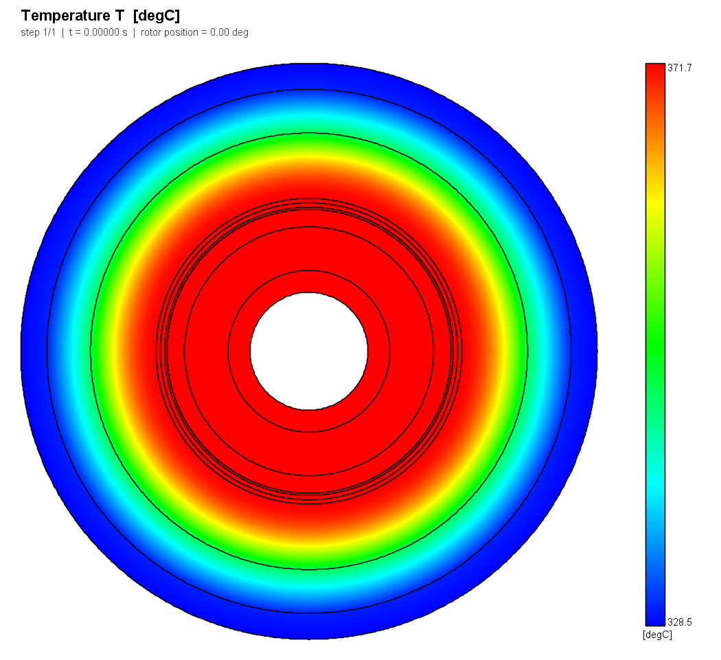
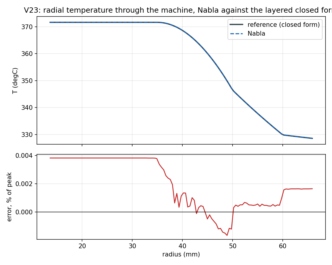
Every station lands inside 0.015 K of the closed form and the radial profile is +0.003 % in L2 — on a stack whose conductivity jumps by a factor of 830 across the airgap, which is the one genuinely hard feature in the problem and the reason the tolerances were set as wide as they were. P1 and P2 agree with each other to -0.00752342 K on the winding and 0.00963499 K anywhere on the profile.

This is a Poisson problem on a smooth domain, so none of that is surprising and none of it is the point of the case; it is the floor the case needed in order for the handoff rows above to mean anything. If the thermal solve had been 1 % off, an 0.02 % conservation result would have proved nothing.

4.3 What the chain actually says about this machine

The winding sits at 365.03 °C, which is -210.03 K of margin against the 155 °C class F hot-spot limit — i.e. 210 K the wrong way. That answer is correct and it is not a defect: V05's "rated point" was chosen to exercise a field comparison, and Iq = 30 A in these slots is 9.44978 A/mm² on the coil-region area — about 1.7 times what this frame can hold continuously, by the estimate two paragraphs down — for 1429.99 W of copper loss against 5.83927 W of stator iron. The machine is producing 37.4119 N·m at 5.87665 kW and 80.3647 % efficiency, and it would do it for about a minute.

A chapter that stopped there would have demonstrated the wiring without demonstrating what the wiring is for. The closed form is linear in the sources and the copper loss goes as I², so the current at which this winding would sit exactly on the class F limit follows in three evaluations: 17.7837 A peak. That is an upper bound — it holds the copper resistivity and the iron loss at their cold values, and both rise with temperature, which is precisely the feedback the uncoupled thermal module does not model.

Two smaller readings worth having:

• The rotor is isothermal. magnet_temp and rotor_surface_temp agree to the last digit printed, because the rotor iron loss is 0.00218232 W — a surface-PM rotor under a sinusoidal drive has nothing to lose. Everything the rotor is at is set by what crosses the airgap, 6.64328 K of it, from the stator.
• The iron-split idealization is worth 0.111725 K. The model puts all of the stator iron loss in the yoke, which is further from the winding than the teeth are. Moving it to the toothed layer in the closed form — both sides are references, so no second solve is needed — moves the winding by that much. On this machine the choice does not matter because the iron loss is 0.4 % of the total; on a high-speed machine it would dominate the chapter.

5. Discussion — where the error comes from

There is very little error to attribute, which is itself the result: the thermal chain has no step in it that loses a percent. Ranked by size:

1. The conservation rows, +0.003 % to +0.017 %. Polygonal circles, as above, plus the contour probe's own segment convention (its samples are per-segment and tagged with the segment's start, so they are integrated as mean x circumference, never as a trapezoid — a trapezoid would have cost 0.14 % here and 0.5 % at V08's sample count).
2. The temperature stations, under 0.015 K. Split between the point probe's linear interpolation (a 1st-order instrument at both element orders — V09 priced it) and the interface geometry.
3. Nothing else is measurable. The P1/P2 difference is 0.008 K, which is below the point probe's own floor.

What would reduce them is not interesting. What would change the answer is: the film coefficient (everything scales with it), the airgap conductivity (the rotor's temperature only), and the slot layer's homogenized conductivity (the winding's rise above the yoke, which is a small part of its rise above ambient). All three are inputs, all three are in thermal_stack.json, and a reader who disagrees with any of them can change one number and re-run.

6. Findings

Both are in the machines module's loss summary — the layer this case reads to get its heat sources — and neither is in a solution. Both were fixed in Nabla on 2026-08-16; each is written below as it was found, with what was changed at the end of it. Full write-ups in case V23.

F1 — IronLoss_FitCurve silently set the iron loss to zero on every shipped material but one

The first version of this case did the documented thing: setRegionMaterial assigns M-19's BH curve but deliberately does not touch Kh/alpha/Ke, so the region property IronLoss_FitCurve exists to re-fit them. Calling it produced IronLossesStator = 0.0 W from a run that converged normally with enableIronLoss still 1.

IronLossCoefficientsFitting returned {0, 0, 0} when the material file has no loss table, and both callers (IronLoss_FitCurve and EnableIronLoss) wrote that onto the region — {0,0,0} is not null, so their guard did not catch it, and calcHystTerm/calcEddyCurrentTerm had no gate of their own. And exactly one file in the shipped soft-magnetic library has a loss table: 1020_steel.csv. M-19, M-15, M-27, M-36, M-43, M-45, M-47, Hiperco-50, Pure Iron, Supermalloy, the US Steel grades — all have an empty #Iron loss section. So the documented way to make the loss coefficients match your material set your iron loss to zero, silently, for every library steel but one. The licence-gated branch of the same function did it too.

Fixed on 2026-08-16. IronLossCoefficientsFitting now returns null on every path that has no fit to offer — the MATERIALS_PRO gate, an absent loss table, an unreadable file, and an optimizer that lands on Kh == Ke == 0 — and all four callers go through one predicate, IronLoss.isUsableFit, which leaves the region's coefficients alone and logs that it did. Checklist.checkIronLoss is the solve-time half: a region asking for a loss it cannot produce is named before the solve rather than after it.

The case's workaround is to not call either, keep the module's own coefficients (fitted to 1020 steel), and report them — stator_Kh = 0.0111887, stator_alpha = 1.59871, stator_Ke = 3.23985e-06 — together with the statement that they belong to a different steel from the BH curve. It is kept after the fix, because the fix makes the two paths agree — calling IronLoss_FitCurve on M-19 now keeps those same 1020 coefficients instead of zeroing them — and keeping the workaround is what makes the numbers on this page the ones its own run produced. The iron loss here therefore still carries that uncertainty; it is 0.4 % of the total, so nothing judged here depends on it, and on a machine where iron loss mattered a material with its own loss table would be the first thing to reach for. extract.py refuses outright on a zero loss channel and its message names F1, because the failure mode is a plausible run.

F2 — PhaseResistance was a factor 2.000 low for a double-layer distributed winding — this was the failing row

Nothing in this machine carries an eddy current and the winding is stranded, so P_joule = 3 I_rms² R_phase is an identity, not an approximation. On the first run the summary reported 1430 W and 529.6 mOhm; the second gives 715.0 W from the first's own current. The ratio was 2.0000, to five figures.

A hand calculation from the slot geometry resolved it in favour of the loss: ~10 mm² of copper per coil side, 20 turns, 100 mm stack → 68 mOhm per side, 16 sides in series per phase → 1.09 Ohm, against the loss-implied 1.059 Ohm and the reported 0.53. So the Joule loss was right — which matters, because it is what this whole chapter rests on — and the reported resistance was half of it.

reconstructPhaseResistanceFromSimCoilsDoubleLayer ended with 0.5 * where both of its single-layer peers ended with 2 *, and accumulated over coils where they break after the first. Two factors of two in one line, so the fix was not the single character it looked like: the three reconstructions needed one convention and a check per winding type. It mattered beyond a summary row, because finalizeImEquivalentCircuit is fed this number as Rs and splits Rr out of the locked-rotor resistance with it.

Fixed on 2026-08-16. The three reconstructions are one private MachinesPostprocessing.reconstructPhaseResistance, on the same side-counting convention as reconstructPhaseSeriesFromSimCoils: R_phase = sum(all sides of the phase) / P² for P parallel branches, with the sides whose periodic images lie outside the sector recovered as sum(matched) * totalSides / matchedSides. The three public entry points now differ only in which end-winding term they add. Single-layer results are unchanged, so the IM equivalent circuit's Rs was never wrong in the other direction. MachinesPostprocessingPhaseResistanceTest asserts 3 I_rms² R_phase == P_joule per winding type — the check this case made from the outside, made from the inside, without a mesh.

The check was written as a judged row, phase_resistance_consistency, rather than as a paragraph, precisely so the case would turn green by itself the day the reconstruction was fixed — which is what happened. The summary now reports 1429.99 W and 1059.25 mOhm, against a loss-implied 1.05925 Ohm, and the row reads its reference of 1 to +0.000 %. Adding it after the run is recorded in the changelog below; it changed no reference and no tolerance that existed before the run.

7. Limitations — what this case does not prove

• It is not a thermal prediction of this machine, and it cannot be. The frame's film coefficient is a fitted input. Every temperature on this page scales with it, and any winding temperature at all can be reached by choosing it. What is validated here is that the chain is wired correctly and that the layered problem is solved exactly — both of which are true for the given h.
• The measured leg the plan asked for is not claimed. The validation plan registers V23 as tier S + M with a 15 K tolerance against a published thermal class or measured rise. V05's machine is a parametric design that was never built; it has no measured rise and no manufacturer's thermal class, and V05 itself ships without a measured leg for a related reason. Fitting h until a winding temperature landed inside a class would be exactly what this dossier exists to prove we do not do. The full sourcing record, and what would unblock it — a published machine with a dimensioned cross-section, winding data, a measured temperature and enough of the cooling arrangement to fix h independently — is in the case's reference notes.
• The chain runs one way, once. Temperatures do not feed back into copper resistivity, magnet remanence or iron-loss coefficients within a run. This is the standing limitation of the thermal module, and this chapter is the case that prices it: the 1429.99 W of copper loss driving a 365 °C winding was computed at the resistivity of a cold one, and would be about 40 % larger if it were not.
• The thermal geometry is not the machine's geometry. Nine annuli are not 24 slots. Circumferential temperature variation — tooth against slot, and the hot spot inside the slot that an insulation class is actually about — is not in this model at all. A 2-D thermal solve of the real cross-section is possible in Nabla and is the obvious follow-on case; what it needs and this one does not is a way to mesh the airgap, which the sliding band makes a hole.
• It proves nothing about transient thermal behaviour, which V08 covers, or about any thermal boundary condition except 22.

8. Reproduce

cd validation
python -m harness.run_case V23              # ~2 minutes, needs triangle.exe
python -m pytest tests/test_analytic_thermal_stack.py -q   # the reference's own tests

The three models are in artifacts/models/; the machine is ../V05_spm_pmsm/design.json and the thermal model is thermal_stack.json, both plain data.

9. Frozen-reference changelog

Each entry says what was true on its own date and is kept as written; the 2026-08-16 entry below therefore records the case failing on the row it had just added, which is the state that day and not the verdict at the top of this page. What changed since is in §6: the defect was fixed and the row turned green on its own, with its reference and its tolerance untouched.

Date	Change	Reason
2026-08-16	three rows added after the first run: phase_resistance_consistency (JUDGED, tol 1 %), phase_resistance_implied_ohm and continuous_current_estimate_A (both report-only). No existing reference or tolerance was touched.	The first run's reported copper loss (1430 W) and reported phase resistance (529.6 mOhm) are inconsistent by a factor of exactly 2.000, which a hand calculation from the slot geometry resolves in favour of the loss (1.09 ohm against the loss-implied 1.059 ohm). That is a defect in a shipped summary number and it was found by reading two rows of one table next to each other, so the check is added as a judged row rather than as a paragraph - a finding that is not a row does not regress when it is fixed. Adding a row is not retuning: it changes no reference and no tolerance that existed before the run, and the case FAILS on it as it stands. See case V23 finding F2. continuous_current_estimate_A was added at the same time because the first run's answer (the winding at 365 degC, 210 K past class F) is correct and is not by itself useful; the current that WOULD sit on the limit is the question the chain exists to answer.