Cable AC loss — skin and proximity effect in a stranded cable

← Back to the examples

What you need to run it: the Python API. The transient run needs nothing beyond that; the time-harmonic run needs Core Pro, and the script says so and exits cleanly rather than failing when the licence is not there. Opening the model and reading results already in it never requires a licence.

What this one is for

Every other example here is a machine. This one is not, and that is the point: it is a plain geometry model — circles, regions, coils and one Dirichlet boundary — built from an empty document by a single script, with no machine module involved anywhere. If you want to see the shape of an API script before committing to a rotor, start here.

The physics it shows is the classical pair that stranded conductors are designed around. Skin effect pushes current away from the middle of each individual strand as frequency rises. Proximity effect is what the strands do to each other: they are driven identically, and they still do not carry or dissipate the same amount, because each one also sits in its neighbours' field. At the settings this model ships with, the second one wins so completely that it empties the middle of the cable.

At a glance

Quantity	Value	Unit
Strands	37 (three honeycomb rings)	—
Strand diameter	1.6	mm
Strand pitch	1.84	mm
Bundle radius	6.32	mm
Outer boundary radius	18.96	mm
Nominal current	100 peak total, 2.70 per strand	A
Frequency	10 000	Hz
Copper conductivity	5.77 × 107	S/m
Skin depth at 10 kHz	0.66, against a 0.80 strand radius	mm
Axial length	1000	mm
Outer shell of strands	3.60 time-harmonic, 3.00 transient	× bundle mean
Innermost strands	0.00 time-harmonic, 0.18 transient	× bundle mean
Mesh	12642 nodes, 25082 elements, P1	—
Wall time, end to end	81 time-harmonic, 136 transient	s

There is deliberately no bundle loss in watts in that table. Further down is why: at these settings the absolute figure this model produces is not a loss, and quoting it would be worse than leaving it out.

What it builds

Thirty-seven copper strands on a hexagonal close-packed lattice — one in the middle and three rings around it — inside a circle of air with A = 0 on the outside. Each strand is its own region with its own conductivity and its own coil, and every coil is driven with an equal share of the cable current, in phase, at the same frequency.

Both the strand count and the strand diameter are parameters at the top of the script. N_RINGS counts honeycomb rings around the centre strand: 0 gives 1 strand, 1 gives 7, 2 gives 19, 3 gives 37, and the geometry, the regions, the coils and the current split all follow from it. Turning a 37-strand cable into a 331-strand cable is one number.

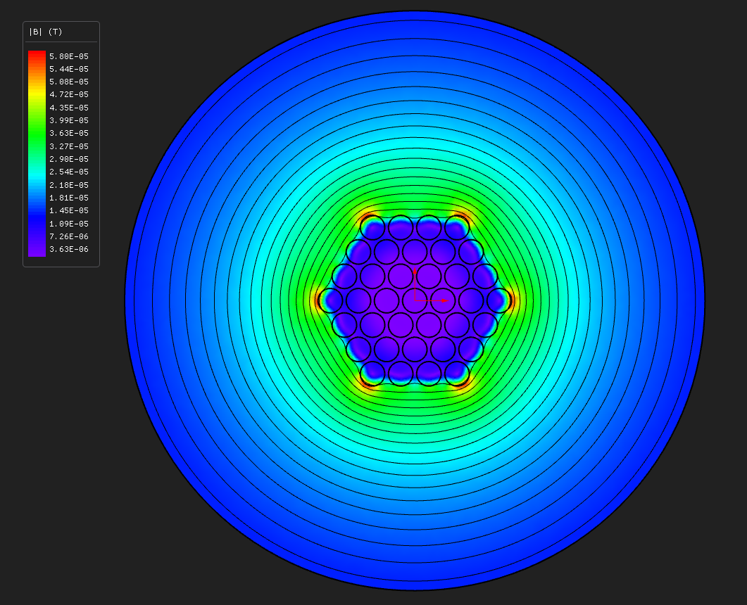
This picture is the whole result. The field does not penetrate the bundle. It peaks in a hot ring on the outermost strands and collapses to nothing a strand or two inside, so the interior of the cable is magnetically shielded by its own outside. Every number below follows from this one picture.

The numbers that say it

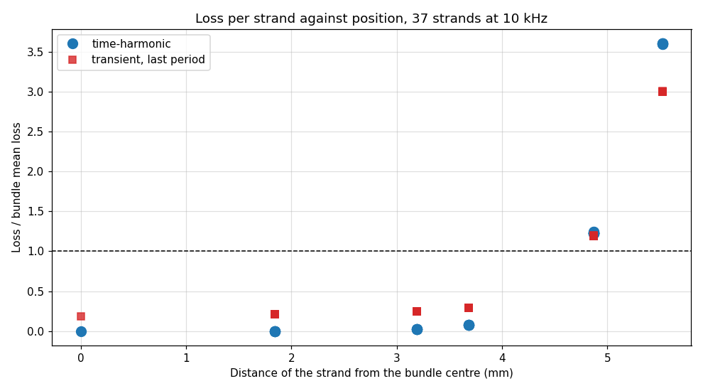
Thirty-seven identically driven strands, and where a strand sits decides everything. The six positions on the geometric lattice fall into shells, and the loss is a staircase down them:

Distance from centre (mm)	Strands	Time-harmonic	Transient
5.52 (outer corners)	6	3.60	3.00
4.87	12	1.23	1.19
3.68	6	0.08	0.29
3.19	6	0.02	0.25
1.84	6	0.00	0.21
0.00 (centre)	1	0.00	0.18

All figures are multiples of the bundle mean. The outermost eighteen strands do essentially all of the work and the inner nineteen are along for the ride — which is the whole argument against building a large conductor as a plain bundle, and the reason litz wire transposes its strands instead of stacking them.

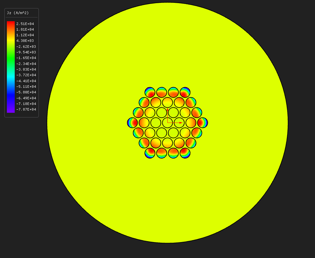
Skin effect within a single strand is real at these settings. The skin depth in copper at 10 kHz is 0.66 mm against a strand radius of 0.80 mm, so a strand is thicker than one skin depth — which it would not be below about 7 kHz. You can see both effects at once in the current density: the outer strands carry a crescent pushed onto their outward-facing side — skin effect distorted by the neighbours — while the interior strands sit nearly flat and nearly empty.

Two solvers, one problem

SOLVER at the top of the script picks one of two runs. They solve the same model and are worth running back to back.

	Transient	Time-harmonic
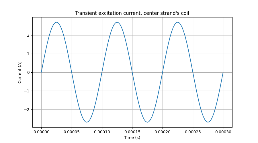
What it does	three periods of the waveform, 40 steps each	one steady-state solve at 10 kHz, replayed as 24 snapshots
Outer shell / mean	3.00	3.60
Centre strand / mean	0.18	0.00
Wall time	136 s	81 s
Licence	none beyond the API	Core Pro

They agree on the shape and differ on how deep the shielded region goes: the frequency-domain run drives the interior strands to essentially zero, the transient leaves them near a fifth of the mean. That gap is the transient's own startup, which three periods at 10 kHz have not fully shed — a steady-state solve has no startup to shed. Raise TRANSIENT_PERIODS and the transient walks toward the frequency-domain answer. It is a useful thing to watch, and a fair warning about how many periods an eddy-current transient needs before it means anything.

Why there is no loss figure on this page

Each strand's coil drives the field directly, with no external circuit — the simplest way to excite a solid conductor in Nabla. The coil prescribes a source current density and the field solve adds the induced reaction on top of it, which is exactly what produces the redistribution above. What it does not do is pin each strand's net current back to the nominal value once that reaction appears, the way a real current source would; that needs the strand wired through the circuit solver, as Nabla's squirrel-cage bars are.

At 2 kHz and seven strands that was a bias. At 10 kHz across 37 mutually coupled strands it is the dominant term: the reaction very nearly cancels the source through most of the bundle, so the model's total comes out at 1.16 mW/m (time-harmonic) and 1.42 mW/m (transient) — against 1.16 W/m of plain DC loss for the same nominal current in the same copper. An AC loss three orders of magnitude below the DC loss is not a loss; it is the statement that the currents in this model are no longer the currents you asked for.

So read this example as a picture of where current goes in a bundle, which it gets right and which is what it is here to show. Do not read a cable rating off it. For AC resistance against closed-form answers, see V12 in the validation dossier; for the same physics with the terminal current actually enforced, the induction-machine examples' rotor bars (E08) are the worked case.

Running it

python cable_AC_loss.py

Set SOLVER = "transient" or SOLVER = "time-harmonic" first — one invocation runs one of them, by design. At the shipped 37-strand size the frequency-domain run takes about a minute and a half and the transient a little over two, mesh included.

Try this next

• Move FREQUENCY_HZ and N_RINGS together. They are the two knobs that decide how dark the middle of the bundle goes, and it takes four short runs to separate them. Centre strand, as a multiple of the bundle mean, from the frequency-domain solver:

  	2 kHz	10 kHz
  7 strands (N_RINGS = 1)	0.88	0.16
  37 strands (N_RINGS = 3)	0.14	0.00

  Neither knob is the whole story: a small bundle at 2 kHz barely grades at all, and either more copper around a strand or a shorter skin depth will bury it.
• Push TRANSIENT_PERIODS up and watch the transient interior fall toward the frequency-domain answer.
• Thicken the strands at fixed total copper area and watch the shielding get worse, not better. That trade is why litz wire exists.

About these numbers

This is a demonstration geometry, not a standard cable, and as the section above says its absolute losses are not engineering figures. Every plot and every number on this page came out of the runs described here, at the settings the script ships with. For accuracy against a stated reference and tolerance, the validation dossier is where that question belongs.

More from this run